Transient Simulation of SHOCK TUBE Using Converge CFD
Aim:
The major objective of this project was to set up Transient Simulation in a Shock Tube using Converge CFD. A shock tube that has a diaphragm in between and the tube is one side filled with high-pressure Nitrogen where the other side is filled with low-pressure Oxygen.
Introduction
The report contains a detailed description of the Shock tube Simulation problem using converge CFD software, solving it using CYGWIN, and post-processing the result using ParaView. This Case Study contains a rectangular duct that has two sections along with a diaphragm in between. A high-pressure reservoir is connected to the low-pressure section
A shock tube is a device for studying shock waves. Prior to starting an experiment, a diaphragm inside the tube blocks any flow. we can increase the pressure on one side, such as with a compressor, and then start the flow by rupturing the diaphragm. The gas expands down the other half of the tube.
1.Geometry Creation
First of all, the Duct geometry along with a diaphragm was imported in Converge CFD software. The geometry was separately prepared using different CAD package ie. Solidworks, then .stl file was imported to Converge Studio to set up the case study.
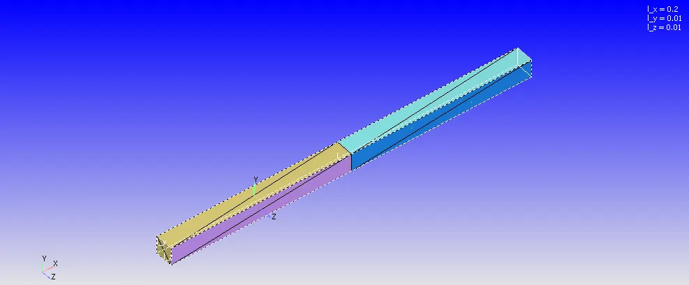
mage 1: Duct geometry along with diaphragm.
The Dimension of Duct is Dx=0.2m, Dy=0.01m, Dz=0.01m.
To create the geometry, the geometry was uploaded from the different CAD software package. Then the geometry clean up was done along with High-pressure regions and Low-pressure regions patch creation for a boundary tagging. All the normal vector were pointing out for this geometry, so we wanted it to point inside and normal to each surface. Normals point the direction of the fluid region generally. The command "Transform" was used to make the normal inside pointing the direction of the fluid region.
2.Boundary Creation
After creating the Duct Geometry, The Boundry tag was created along with different boundary id and coloring. A total of 6 different boundaries tag was created for so many different split triangles of the duct with each face split into multiple triangles. To create the boundaries naming, the "Boundary" command in the "Geometry" dock was used, and then the faces were appointed to appropriate tags along with id.
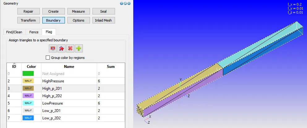
Image 2: Boundary creation representing the different id and color.
The five different boundaries were High pressure, High_p_2d_1, High_p_2d_2, Low pressure, Low_p_2d_2, and Low_p_2d_1.
3.Case-Study Setup
The various parameter was considered while setup this case study. The case study setup dock was used to set up the problem which appears on the right-hand side of the converge studio.
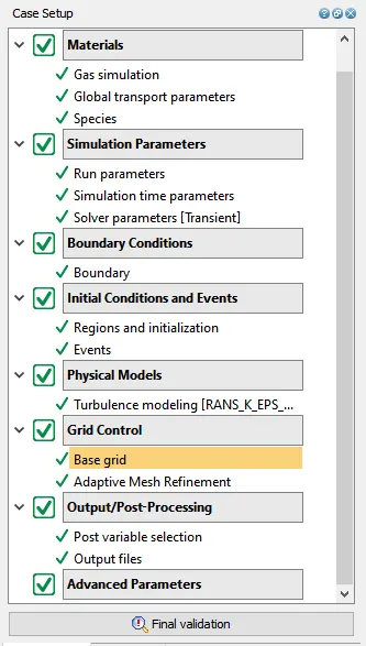
Image 3: Case Setup Dock.
3.1 Application Type:
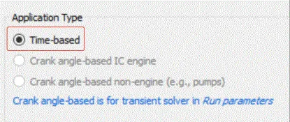
In order to run a steady-state simulation, firstly, under the Application type in the setup tree, a "Time-based" simulation must be selected.
3.2 Materials:
Under the material tab "Gas simulation" was selected and "Air" as a predefined mixture.
Gas: Air
Global Transport Parameters: Fixed value
by default, the following value is considered.
Prandtl Number : 0.9
Schmidt Number : 0.78
Species: Oxygen-O2 & Nitrogen-N2
3.3 Simulation Parameters
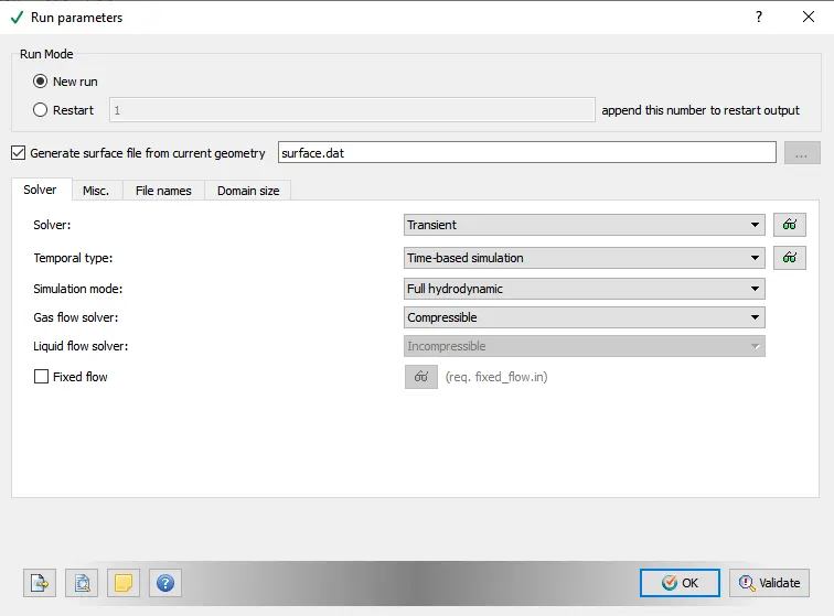
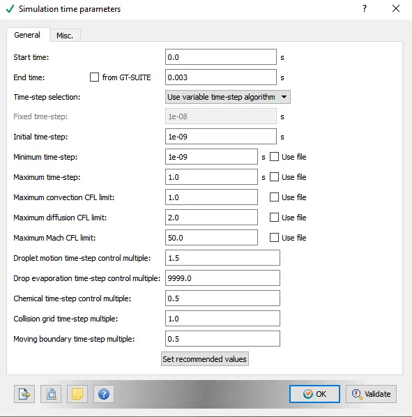
The Transient solver was selected for running this case study along with a "Density-based" solver.
3.4: Boundary Conditions
In this tab, The volumetric region and physics for each boundary were defined.
| Boundary_Name | Boundary_Type | Paramter_Defined | Boundary ID |
| 1.High pressure | Wall | Slip | 2 |
| 2.High_p_2d_1 | Wall |
Slip |
3 |
| 3.High_p_2d_2 | Wall | Slip | 4 |
| 4.Low pressure | Wall |
Slip |
5 |
| 5.Low_p_2d_1 | Wall | Slip | 6 |
| 6.Low_p_2d_2 | Wall | Slip | 7 |
3.5: Initial Conditions and Events
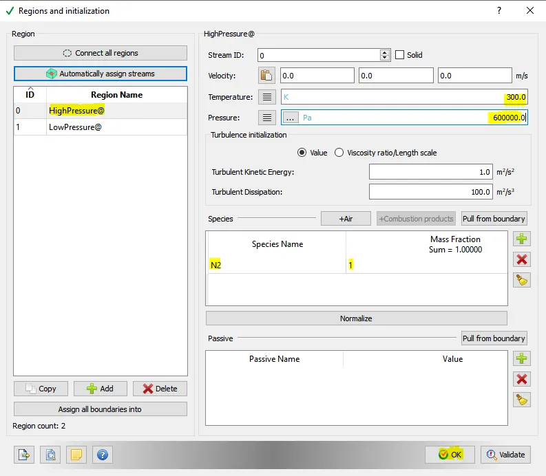
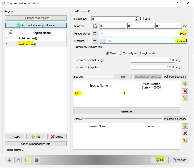
Two Volumetric Region was created in order to assign this to all the boundary tag.
Region one: High-Pressure Region
Species:- N2 (1)
Pressure:6,00,000.0Pa
Temperature:300K
Region Two: Low-Pressure Region
Species:- O2 (1)
Pressure:1,01,325.0Pa
Temperature:300K
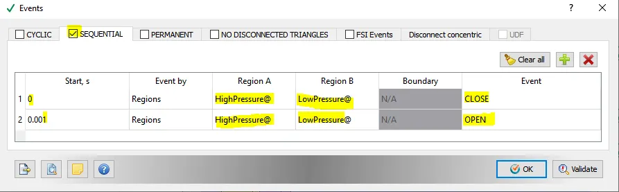
Concept of Event in Converge Studio:
When 2 regions are in contact with each other with no boundary in-between them, it is necessary to use events. The events flag creates triangles in the place between the 2 regions called as disconnect triangles.
The events flag can be turned on before the case set-up, by navigating to the initial conditions window and checking the events option.
3.6: Physical Models
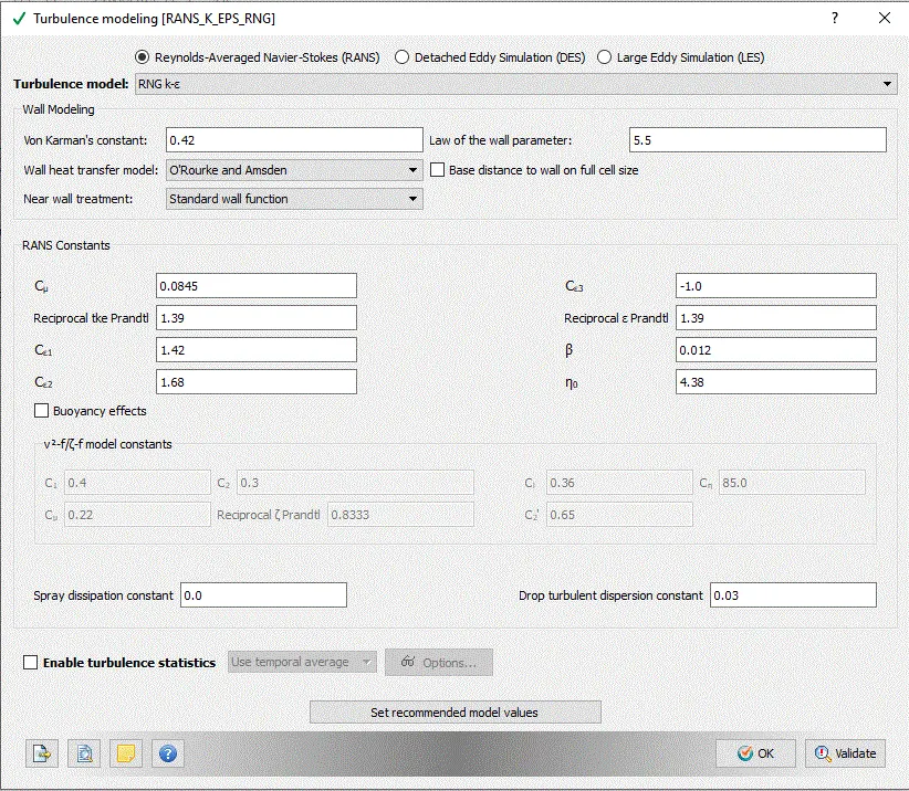
A turbulent model was selected out of so many models.
3.7: Grid Control
Grid Size
Base mesh sizes are,
| S.No. | Dx(m) | Dy(m) | Dz(m) |
| 1 | 0.001 | 0.001 | 0.001 |
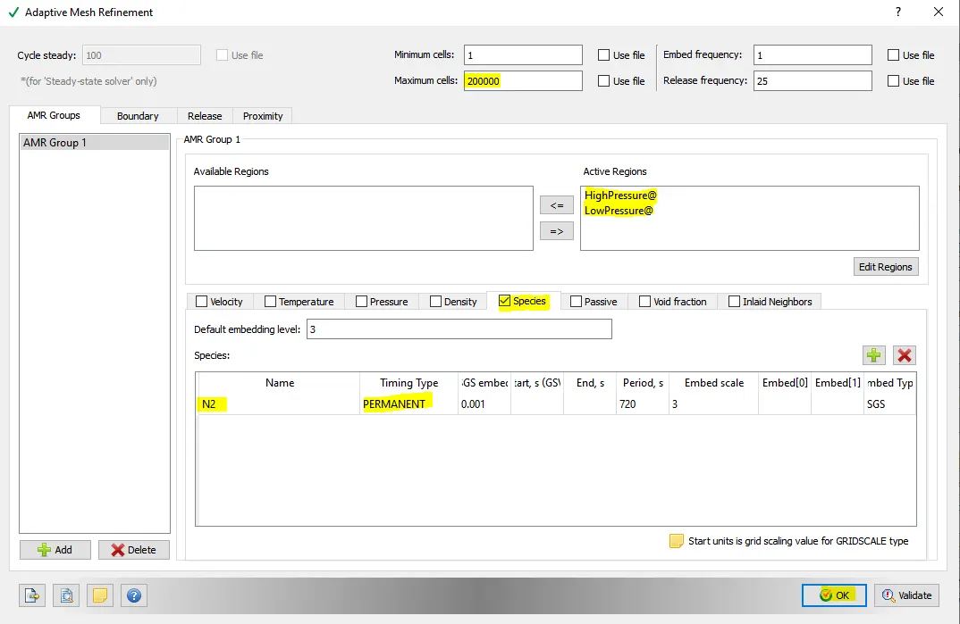
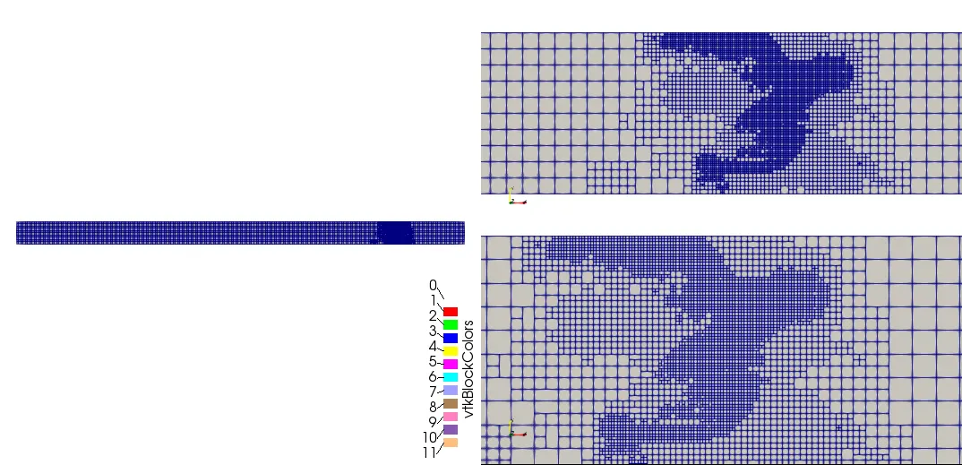
The Adaptive mesh refinement was selected:
3.7 Output/Post-Processing
Post-Variable Selection- Existing value
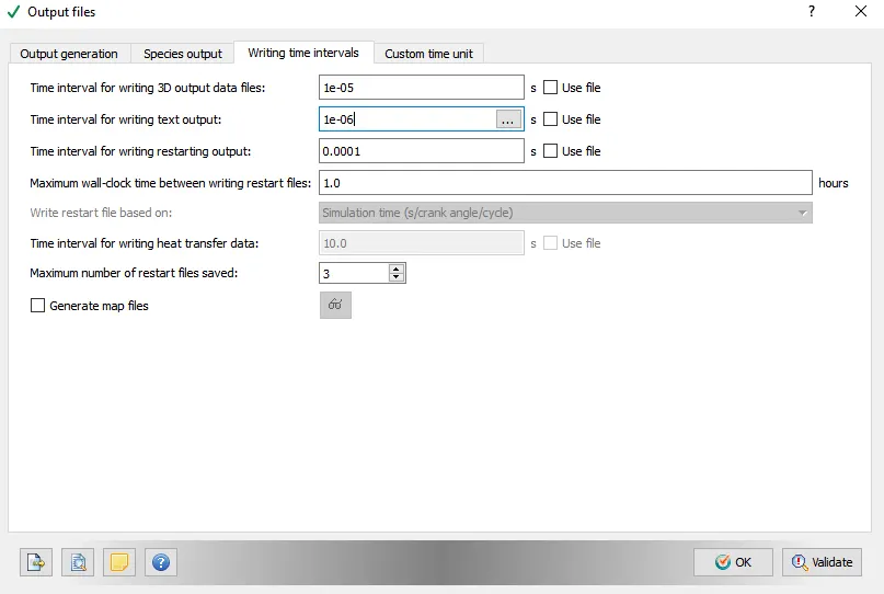
Output Files- Time interval for writing 3D output files-1e-05 s
The time interval for writing restart files -0.0001s
The case study was solved using CYGWIN and the post-processing was done in ParaView.

For post converting we used the following command

SIMULATION RESULTS
Mesh Size
Case Study 1: dx=dy=dz=2e-3 m
Mesh
T Step=0

T Step=20

T Step=30

T Step=40

T Step=50

T Step=60

T Step=70

T Step=80

T Step=90

T Step=100

T Step=110

T Step=120

Contours
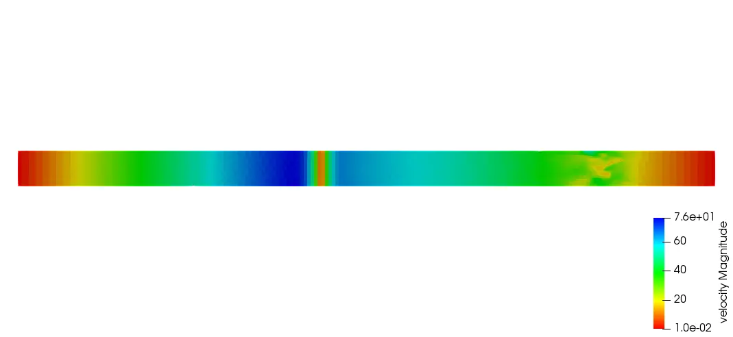
Velocity Contour
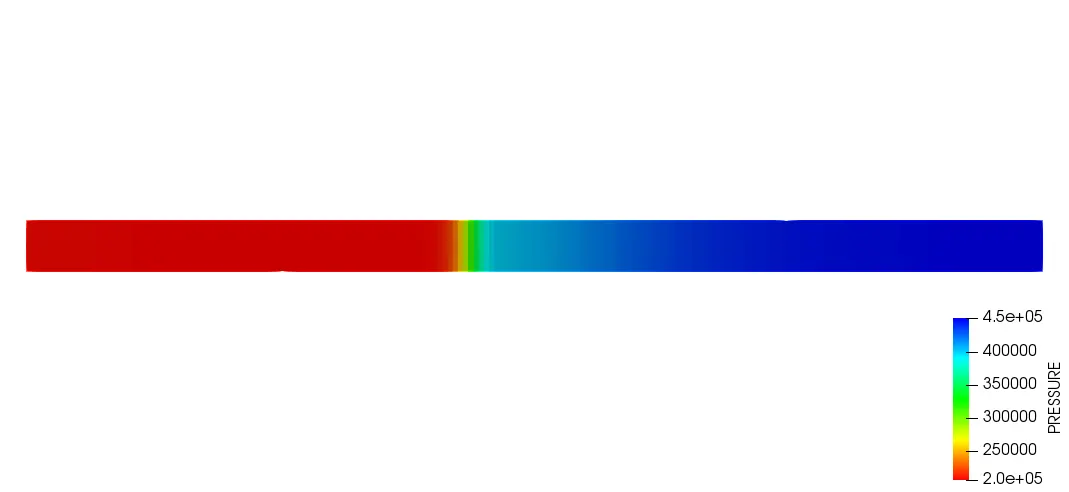
Pressure Contour
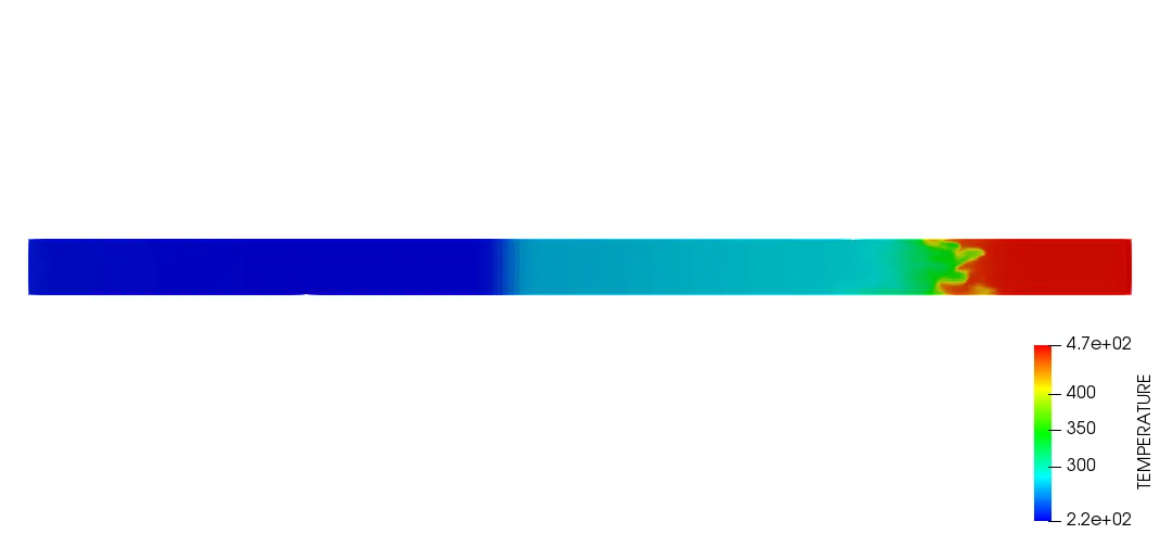
Temperature Contour
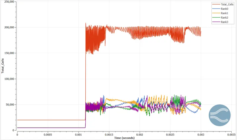
Cell Count
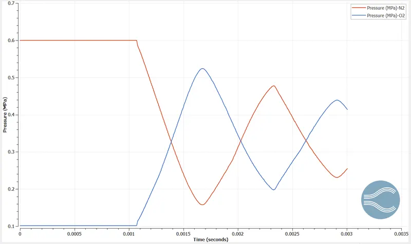
Pressure Plot
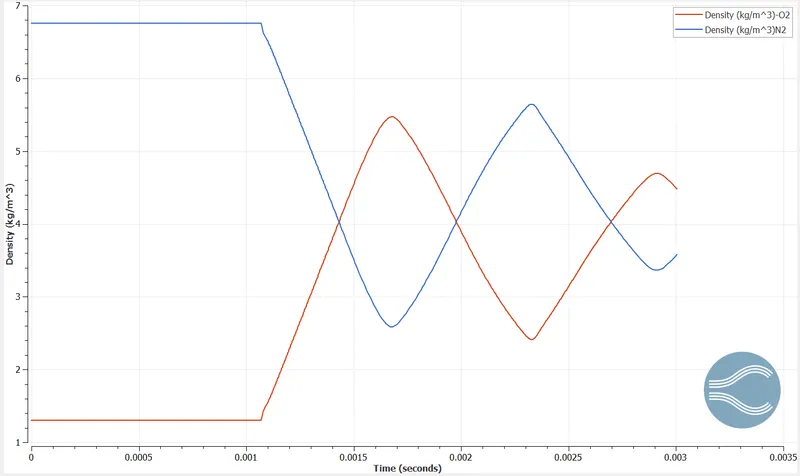
Density
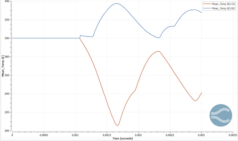
Mean Temperature
Conclusion
The low-pressure O2 is compressed by high-pressure N2 gas, which is subsequently recirculated and the low-pressure gas flows through the N2. We can learn about gas compressibility and flow by working through this situation. The cell count is constantly changing due to adaptive mesh refinement as the shock tube expands and contracts. The pressure plot shows that over a period of time, both species will have a common pressure, since one is growing and the other is dropping in relation to time. Temperatures will vary at first, then return to equilibrium over a period of time.
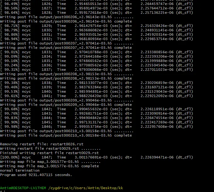
As the mesh was very refined so the computational time was little more and was fond to be 9231 sec.
The Case Study can be downloaded from here: Shock Tube