Rayleigh Taylor Instability Using Ansys Fluent
Aim
The major objective of this project is to set up a Transient-Multiphase simulation to observe Rayleigh Taylor Instability using Ansys Fluent.
Introduction
Multiphase flow Engineering is a very important topic of interest when we want to analyse different phases with different state or phases. Phases can be a combination of solid, liquid or gas.
There are three types of interphase in Multiphase engineering:
1. Separated Phase
2. Mixed Phase
3. Dispersed Phase
Earlier black-box approach model did not provide information about flow visualization.

There are many flow regimes that can be seen in multiphase flow engineering.
The details of different flow regimes are represented in the flow regime map for various setup of control parameters but for a specific problem.
The Rayleigh–Taylor instability or RT instability is the instability of an interface between two fluid of different densities which occurs when the lighter fluid is pushing the heavier fluid.


The Rayleigh-Taylor Instability arises from small wavelength disturbance or perturbation at the interface (A) which further grows into allover mushroom shapes spikes and bubble (B) and these fluid structures interact due to bubble merging and competition (C) eventually developing into a mixing region (D)- Rho(2) represent the high-density fluid, vice versa. gravity plays an important role downward and the system is RT unstable.
Saffman-Taylor Instability also known as viscous fingering. It is the formation of patterns in a morphologically unstable interface between two fluids in a porous medium. This process occurs when a less viscous fluid is injected displacing a more viscous fluid in the inverse situation, with the more viscous displacing the other, the interface is stable and no instability is seen. Essentially the same effect occurs driven by gravity (without injection) if the interface is horizontal and separates two fluids of different densities, the heavier one being above the other: this is known as the RT instability.
Richtmyer–Meshkov instability (RMI)-occurs when two fluids of different density are impulsively accelerated. Normally this is by the passage of a shock wave. The development of the instability begins with small amplitude perturbations which initially grow linearly with time. This is followed by a nonlinear regime with bubbles appearing in the case of a light fluid penetrating a heavy fluid, and with spikes appearing in the case of a heavy fluid penetrating a light fluid. A chaotic regime eventually is reached and the two fluids mix. This instability can be considered the impulsive-acceleration limit of the RT instability.
Kelvin–Helmholtz instability typically occurs when there is Velocity shear in a single continuous fluid, or additionally where there is a velocity difference across the interface between two fluid.
Plateau–Rayleigh instability, often just called the Rayleigh instability, explains why and how a falling stream of fluid breaks up into smaller packets with the same volume but less surface area

1.Geometry Creation Using Ansys Design Modular
First of all, The Rectangular domain shaped body geometry was created using a separate CAD package i.e. Solidworks. Then the same geometry was imported in Ansys workbench for generating the fluid flow domain volume to define the boundary conditions and further proceed with Pre Processing, and post-processing the results. The Shared Topology was enabled to define the interface between two fluid.
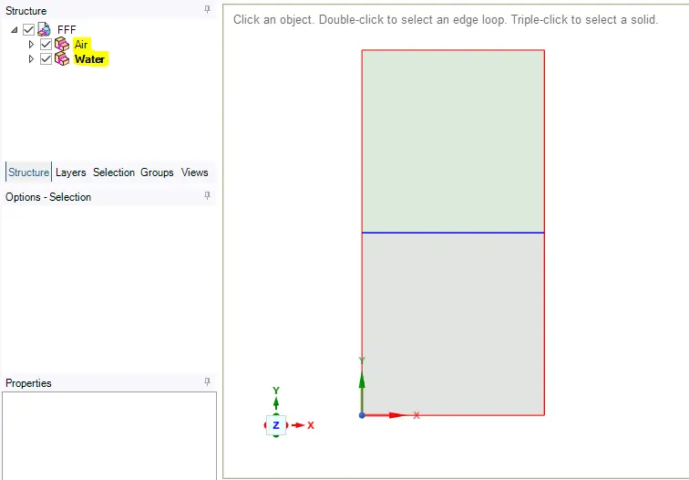
Pre Processing
2. Boundary Creation and Meshing
After the control volumes are perfectly created the boundary tags were created in order to assign the different boundary conditions ie. velocity, temperature, or some other physics. For this geometry, 2 different boundary tags or names were created that were used earlier to assign the boundary condition. The 2 names are Air and water. No Inlet or outlet patches or BC was created for this problem.
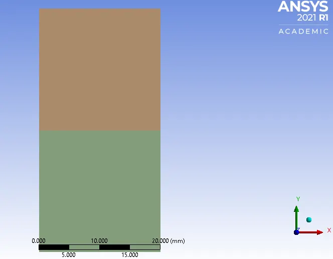
Meshing
As the Greomtry was very simple and a simple Quad Mesh was created using the Automatic Meshing option in Ansys.
Mesh 1 With 0.15mm base Size
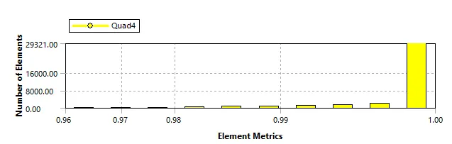
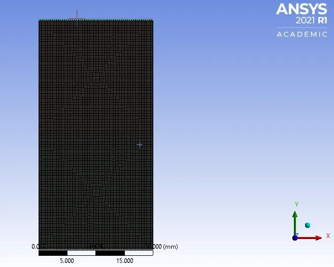
Mesh 2 With 0.3mm base Size
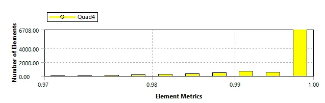
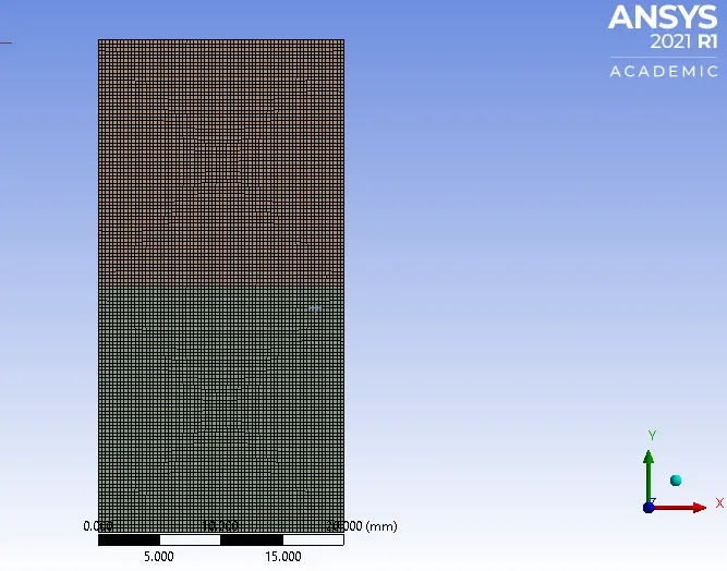
Mesh 3 With 0.5mm base Size
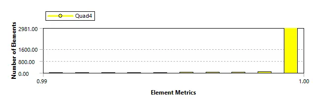
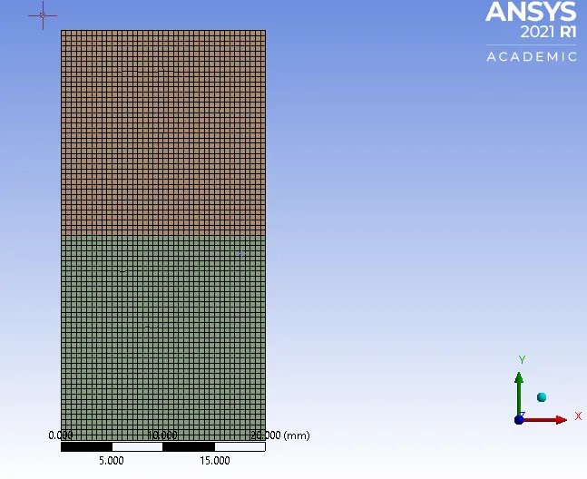
Mesh Parameters & Information
| Element Size | No. of Elements | No of Nodes | |
| Coarse Mesh | 0.50mm | 3200 | 3321 |
| Medium Mesh | 0.30mm | ||
| Fine Mesh | 0.15mm | 35378 | 35778 |
Meshing is very important so that for really small infinitesimal control volumes the equation of fluid flow can be used in order to generate useful information.
3. Case Study Setup
For setting up the case study Ansys Fluent was used in order to simulate the case study.
The various parameter was considered while setup this case study. The case study setup dock was used to set up the problem which appears on the left-hand side of the Ansys Fluent
Gravity was Enabled for this problem as that is very important paramter for RT Instability.
| S.No. | |||
| 1 | Models | ||
|
Viscous Model-Laminar Model |
As the the simualtion was due to free fall of gravity | ||
| 2 | Material |
Air (N2:O2::23%:77%) Water |
Air was used as the Primary Fluid Water was used as secondary fluid. |
| 3 | Cell Zone Condition | Control Volume Region was set to Air | The flow inside the Control volume wanted it to be only air. |
| 4 | Boundary Conditions | No Inlet or Outlet | |
| The side walls were set to stationary walls with no slip BC |
5. Solution
For the Solution Residuals Monitor, the Magnitude was changed to 1e-6 to get less error with more accuracy.
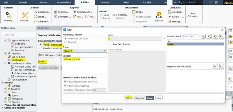
Hybrid Intilizization was used in order to initialize this simulation.
The Water region was patch with the material properties with the Volume fraction of water as one.
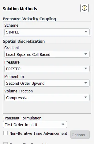
For better Convergence result following schemes were used for this simulation:
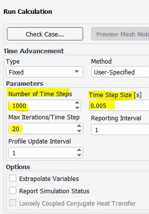
As this was Transient Simulation so the Simulation was run for 1000 iterations and the results were generated easily.
Case Study 1: Primary Phase Air and Secondary Phase Water
Rayleigh Taylor Instability 0.5mm Mesh 40X20mm Domain
Residual Plot
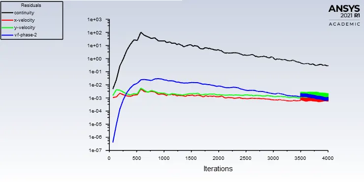
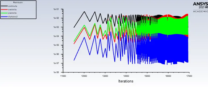
Case Study 2: Primary Phase Air and Secondary Phase Water
Rayleigh Taylor Instability 0.3mm Mesh 40X20mm Domain
Residual Plot
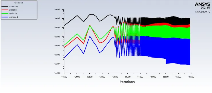
Case Study 3: Primary Phase Air and Secondary Phase Water
Rayleigh Taylor Instability 0.15mm Mesh 40X20mm Domain
Residual Plot
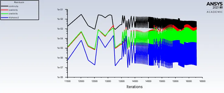
Case Study 4:
Rayleigh Taylor Instability 0.15mm Mesh 40X20mm Domain with `rho=400(kg)/m^3 " " mu=0.001 kg/(m-s)`
Conclusion
From the above cases it can be concluded that Rayleigh Taylor Instability is observed at the interface of both the phasses, lower density luid pshues a higher density fluid due to formation of chock waves at interface. formation of air bubble takes placethat compresses the heavy fluid around itdue to which shock waves of multidimensional fashion are observed and gets more stronger with respect to time.
It can also be noticed that more we refine the mesh more smooth volume of Fraction contour is observed and instabilities can be observed more clearly. The transformation from instable to stable equillibrium can be seen duw to transient simualtion.
When the user defined material was used the system becomes more unstable due to lower desnity of fluid as compared with other cases where water is used as heavier liquid. When the heavier fluid was used the system reaches the equlibrium state fast as compared with under defined material with lower density.
Steady State and Transient Simulation
Steady State Simulations are the simulation that we run if are just interested in the end result and not we are not interested on how those results are getting formed with time. The fluid properties do not change with respect to time or there are no time derivative terms in the equations of motion that govern the fluid flow.
If we want to see how results are changing w.r.t time and how the solution is getting formed over time then we need to run the TRANSIENT STATE SIMULATION.
The time is in Cycles for STEADY STATE SIMULATION whereas time is in Seconds for TRANSIENT STATE SIMULATION.
To capture the instability for this problem Transient Simulation was perfomed for different timestep and the animation file was generated.
Atwood Number
Atwood number is a important dimensionless number in fluid dynamics used to study the hydrodynamics instabilities in density of startified flows. It is generally the dimensionless density ratio and is given by:
`A=(rho_1-rho_2)/(rho_1+rho_2)`
Where
`rho_1 " is the density of Heavier Fluid"`
`rho_2 " is the density of Lighter Fluid"`
Atwood Number for this case:-
`A=(1000-1.25)/(1000+1.25)=0.9975`
`rho_1=1000(kg)/m^3- " Water density ( Heavier Fluid)"`
`rho_2=1.25(kg)/m^3- " Air density ( Heavier Fluid)"`
Atwood Number for Second case:-
`A=(400-1.25)/(400+1.25)=0.9937`
`rho_1=400(kg)/m^3- " Water density ( Heavier Fluid)"`
`rho_2=1.25(kg)/m^3- " Air density ( Heavier Fluid)"`
Note:
If Atwood Number is Close to 0, Rayleigh Taylor Instability Flow takes in form of Symmetric "Finger" of Fluid.
If Atwood Number is Close to 1, the much lighter fluid "below" then Rayleigh Taylor Instability Flow takes in form of unSymmetric of Fluidas the hevier takes the form of larger bubble like plumes.