Prandtl Meyer Shock Problem Using Converge CFD
Aim:
The major objective of this project was to Simulate Prandtl Meyer Shock Problem Using Converge CFD & to study the Effect of the SGS parameter on shock location along with other useful data.
1. Simulate the SuperSonic and SubSonic flow through a duct which has a sharp corner.
2. Study the effect of Shock formation when the Parameter such as grid and SGS are changed.
3. Study the Effect of the SGS parameter on shock location
Introduction
The report contains a detailed description of the Prandtl Meyer Shock Problem using converge CFD software, solving it using CYGWIN and post-processing the result using ParaView. Various steps are discussed in this report while making a case set up for this case study. This report contains a detailed description of the case study with grid sizing, line plots, the effect of SGS parameter, and contours.
Theory
What is a Shock wave?
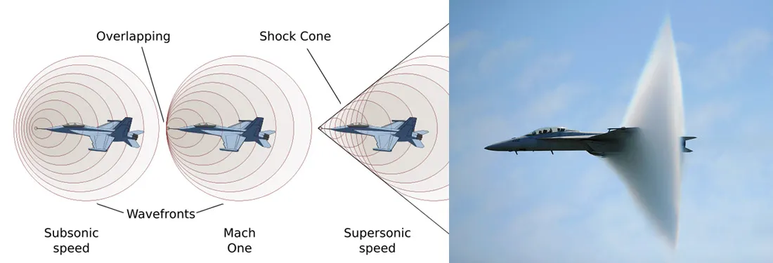
Shock is a type of continuous propagating disturbance that occurs when a state of supersonic speed is achieved in that medium ie. faster than the speed of sound and it also carries energy and can propagate through a medium similar to an ordinary wave. But in the shock wave, there is an abrupt change in pressure, temperature, and the density of the medium.
It is basically a strong pressure wave in any medium may be air or water. The are many examples, we can see in our daily life like supersonic aircraft, supersonic bullet and so many. In a simple way, Shock waves are large amplitude pressure waves produced by an object moving faster than the speed of sounds like a boat or plane, or other things such as an explosion, lightning or even a moving piston.
Prandtl-Meyer Expansion Fan
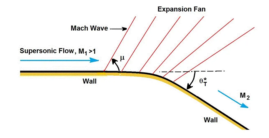
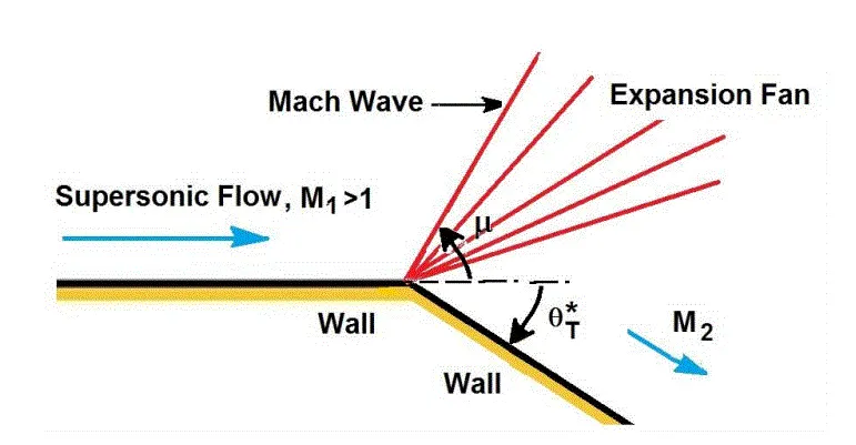
A supersonic expansion fan, technically known as Prandtl–Meyer expansion fan, a two-dimensional simple wave, is a centered expansion process that occurs when a supersonic flow turns around a convex corner. The fan consists of an infinite number of Mach waves, diverging from a sharp corner. When a flow turns around a smooth and circular corner, these waves can be extended backward to meet at a point.
Shock Flow Boundry Conditions
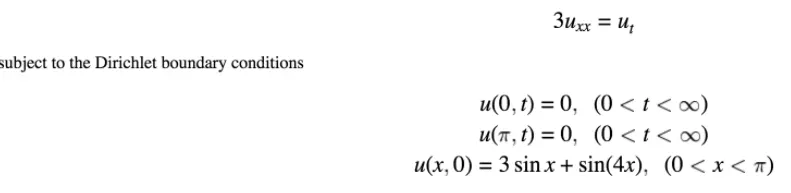
1.Dirichlet Boundary Condition
In Dirichlet Boundary Condition, The value of the function is specified at the boundary
y=f
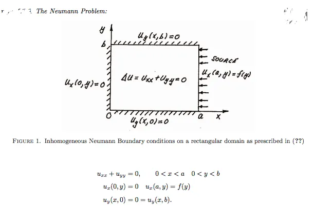
2.Neumann Boundary Condition
In Neumann Boundary Condition, the value of the normal derivative of a function is specified.
`frac {dy}{dn}=f`
3. Robin Boundary Condition
It is the combination of both the above boundary, specified at both ends.
`c0.y +c1. frac{dy}{dn}=f`
4.Mixed Boundary Condition
One end there is Dirichlet boundary condition and on the other end, there is a Robin boundary condition.
Why is the Neumann Boundary condition used for Supersonic Outlets?
it's Because the value of all the variables ie. the pressure, velocity, temperature, mach no. are also not available before solving the problem. so something is specified at a supersonic outlet and all are extrapolated from the domain interior. only the normal derivatives of the variable are specified as zero gradients.
However, if any pressure values or velocity is specified at the outlet the solution will not converge and become unstable.
1.Geometry Creation
First of all, the Duct geometry along with sharp turn was imported in converge CFD software. The geometry was separately prepared using different CAD package ie. Solidworks, then .stl file was imported to Converge Studio to set up the case study.
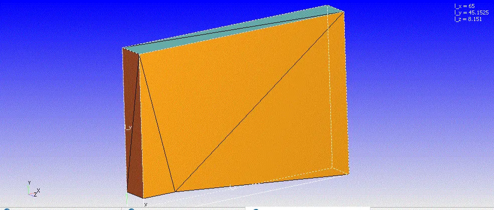
Image 1: Duct geometry along with Sharp corner.
*Each face of the step was split into multiple triangles.
The Geometry can be downloaded from this link: Geometry
To create the geometry, the geometry was uploaded from the different CAD software package. Then the geometry clean up was done along with inlet and outlet patch creation. All the normal vector were pointing out for this geometry, so we wanted it to point inside and normal to each surface. Normals point the direction of the fluid region generally. The command "Transform" was used to make the normal inside pointing the direction of the fluid region.
The Geometry was a check for if the geometry has any open surface.
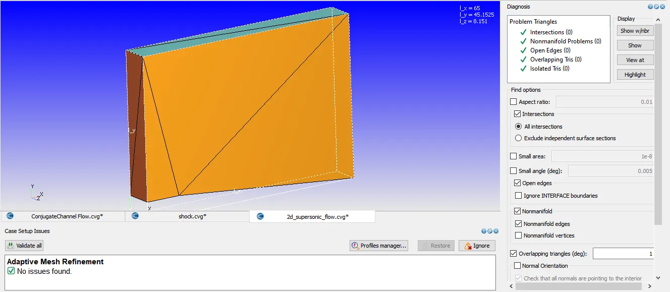
Then the normal edge checked and from the diagnostic dock, everything was checked.
2.Boundary Creation
After creating the Duct Geometry, The Boundry tag was created along with different boundary id and coloring. A total of 5 different boundaries tag was created for so many different split triangles of the duct with each face split into multiple triangles. To create the boundaries naming, the "Boundary" command in the "Geometry" dock was used, and then the faces were appointed to appropriate tags along with id.
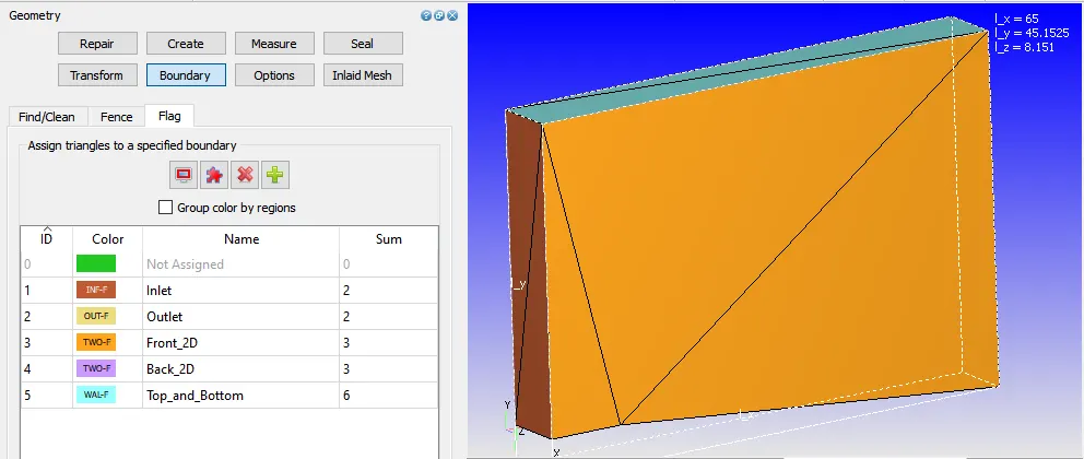
Image 2: Boundary creation representing the different id and color.
The five different boundaries were Inlet, Outlet, Top_and_Bottom, Front_2D, and Back_2D.
3.Case-Study Setup
The various parameter was considered while setup this case study. The case study setup dock was used to set up the problem which appears on the right-hand side of the converge studio.
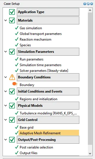
Image 3: Case Setup Dock.
3.1 Application Type:
In order to run a steady-state simulation, firstly, under the Application type in the setup tree, a "Time-based" simulation must be selected.
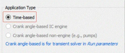
3.2 Materials:
Under the material tab "Gas simulation" was selected and "Air" as a predefined mixture.
Gas: Air
Global Transport Parameters: Fixed value
by default, the following value is considered.
Prandtl Number : 0.9
Schmidt Number : 0.78
Species: Oxygen-O2 & Nitrogen-N2
Reaction Mechanism (mech.dat) was selected for this problem.
3.3 Simulation Parameters
The Steady-State solver was selected for running this case study along with a "Density-based" solver.
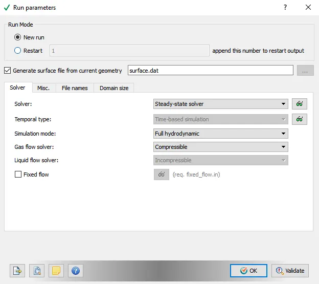
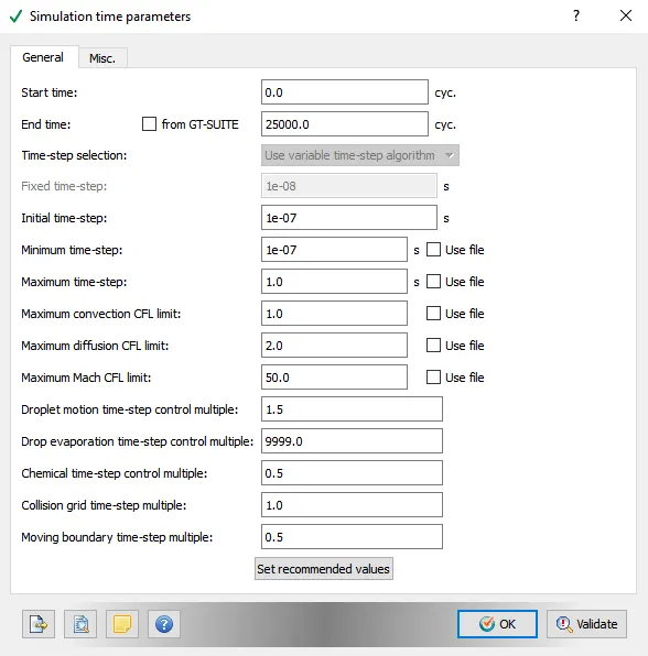
3.4: Boundary Conditions
In this tab, The volumetric region and physics for each boundary were defined.
| Boundary_Name | Boundary_Type | Paramter_Defined | Boundary ID |
| 1.Inlet | Inflow | 680m/s at 286.1k | 1 |
| 2.Outlet | OutFlow |
Dirichlet Boundary Condition Temperature Back Flow is 300K |
2 |
| 3.Front_2D | Two_D | 3 | |
| 4.Back_2D | Two_d | 4 | |
| 5.Top_and_Bottom | Wall | Slip | 5 |
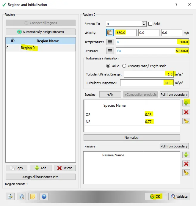
3.5: Initial Conditions and Events
Volumetric Region was created in order to assign this to all the boundary tag.
Species:- O2 (0.23) & N2 (0.77)
Pressure :50,000Pa
Temperature:300K
Velocity:(680, 0, 0)m/s
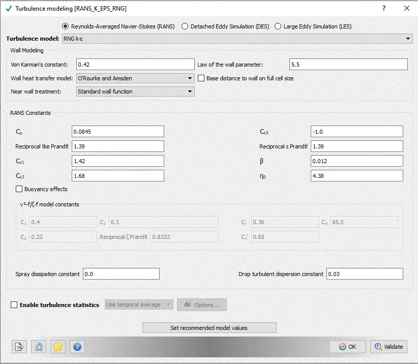
3.6: Physical Models
A turbulent model was selected out of so many models.
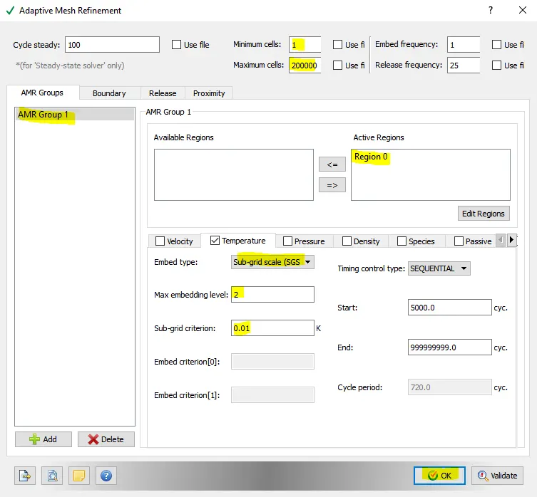
3.7: Grid Control
The case study was run using a 4 fine SGS parameter size and at supersonic & subsonic speed. So different case study was set up in order to study the effect of value when the mesh is more refined.
The Adaptive mesh refinement was selected
Base mesh sizes are,
| S.No. | Dx(m) | Dy(m) | Dz(m) | Speed(m/s) | SGS |
| 1 | 0.8 | 0.8 | 0.8 | 680 | 0.05 |
| 2 | 0.8 | 0.8 | 0.8 | 680 | 0.01 |
| 3 | 0.8 | 0.8 | 0.8 | 680 | 0.1 |
| 4 | 0.8 | 0.8 | 0.8 | 100 | 0.05 |
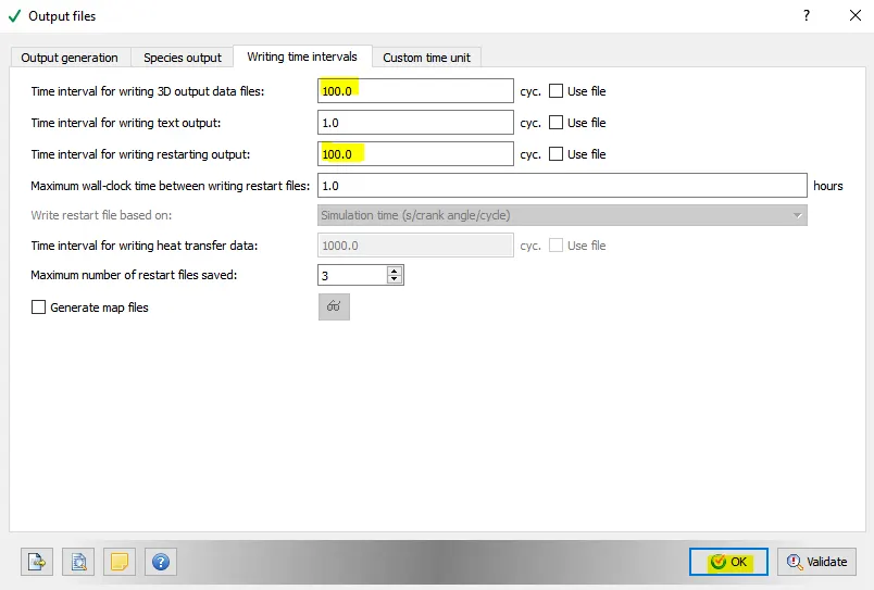
3.7 Output/Post-Processing
Post-Variable Selection- Existing value
Output Files- Time interval for writing 3D output files-100 s
The time interval for writing restart files -100s
The case study was solved using CYGWIN and the post-processing was done in ParaView.
SuperSonic Flow
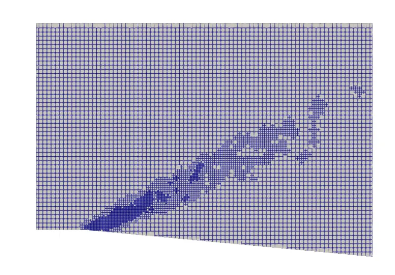
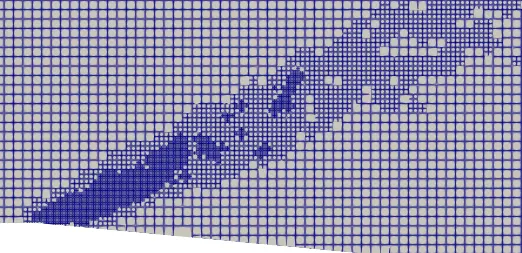
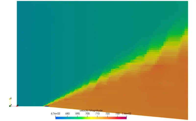
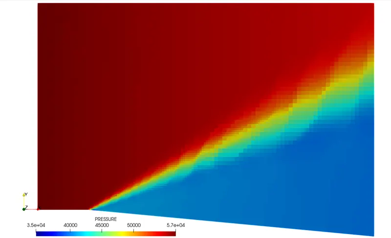
Case Study 1: Grid Size 0.8m SGS 0.05 Velocity 680m/s
Mesh Quality
Contour Plots
Velocity Contour
Pressure Contour
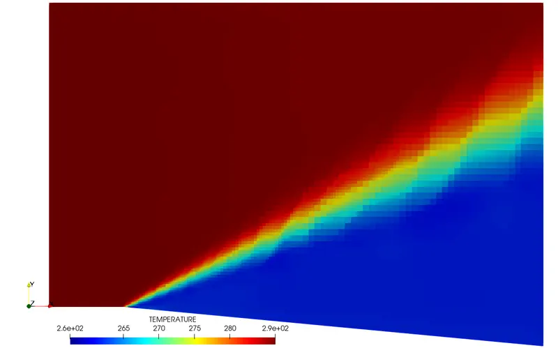
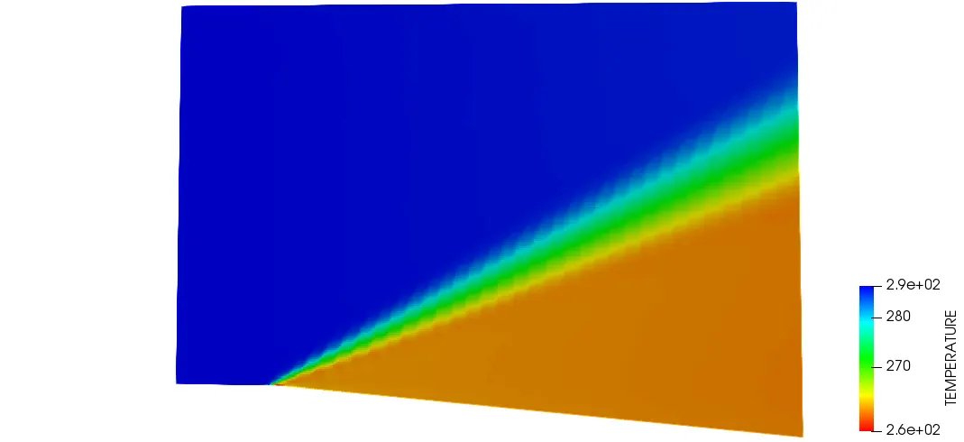
Temperature Contour
Line plots
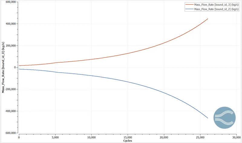
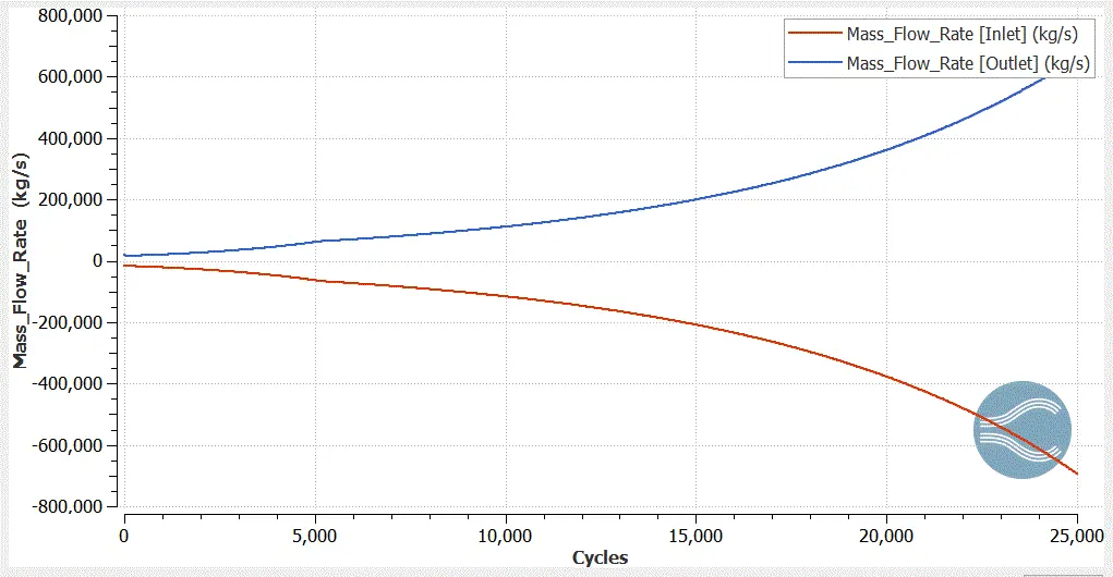
Mass Flow Rate
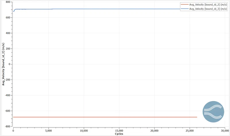
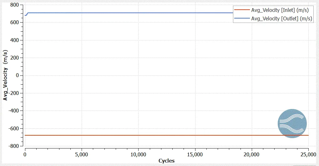
Velocity Plot
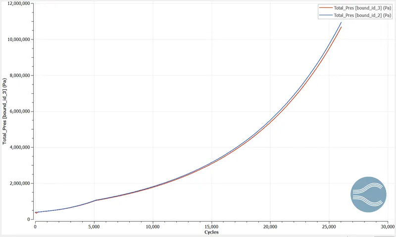
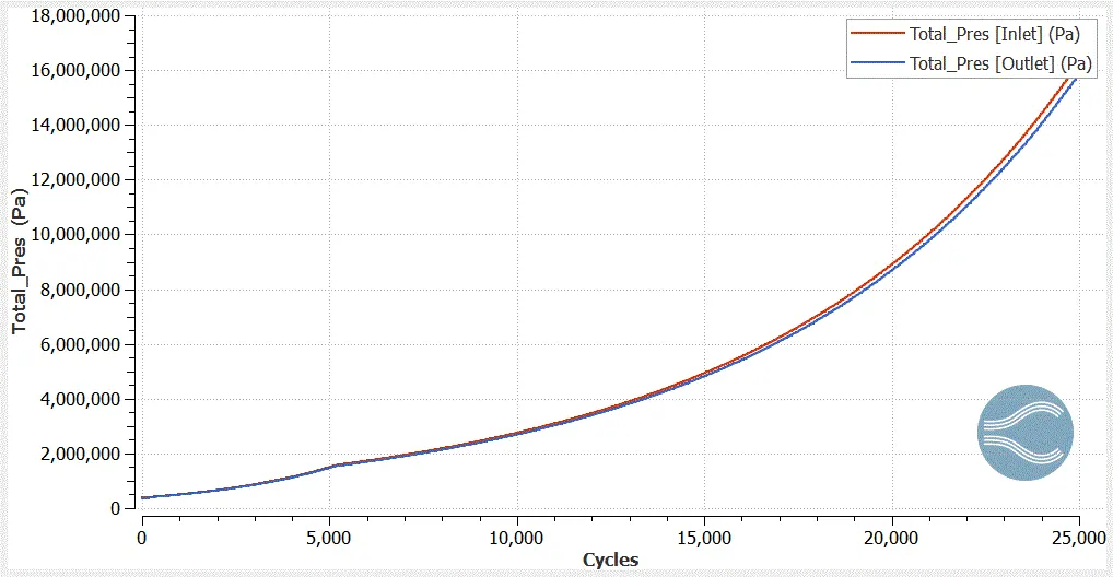
Pressure Plot
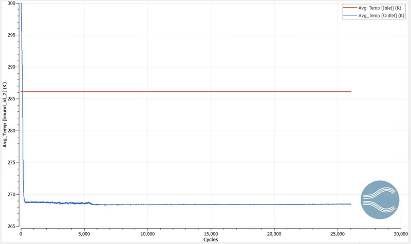
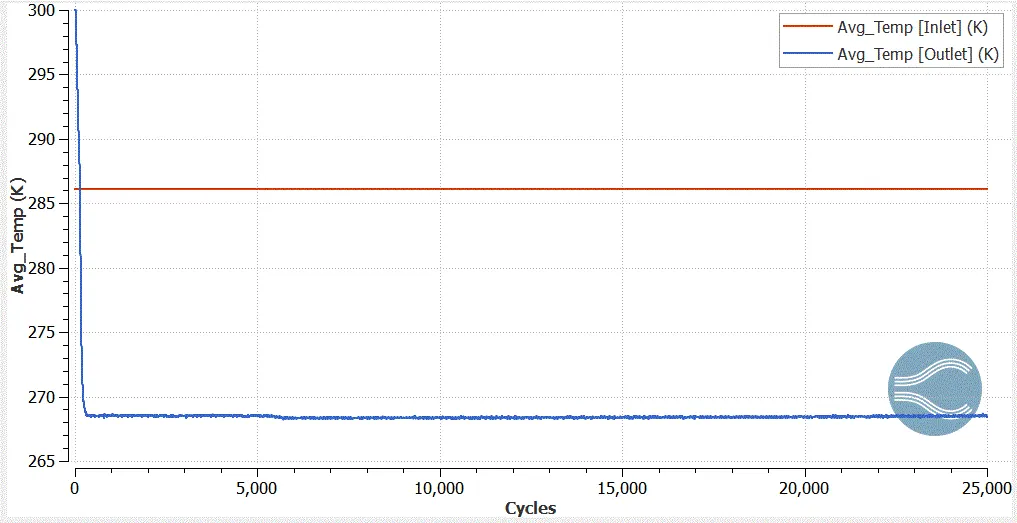
Temperature Plot
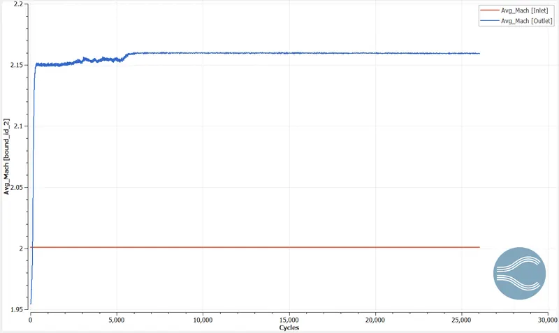
Mach Number Plot
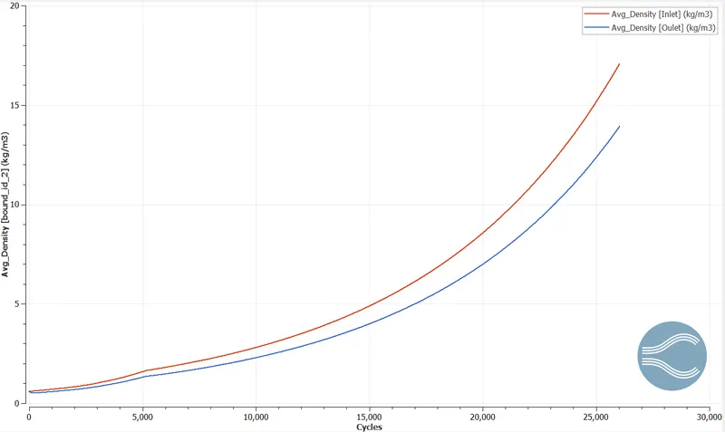
Density Plot
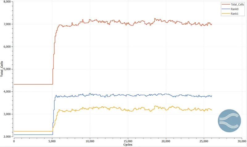
Cell Count
Animation
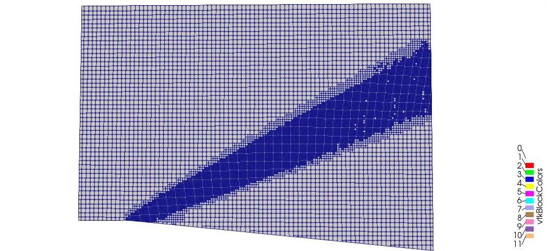
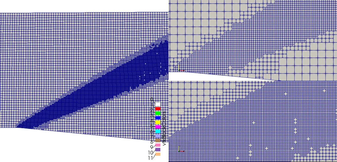
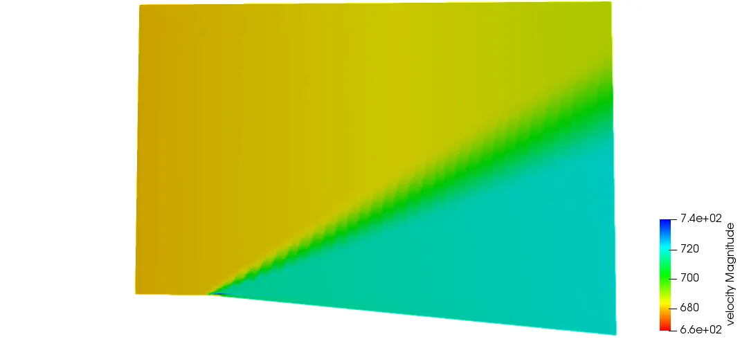
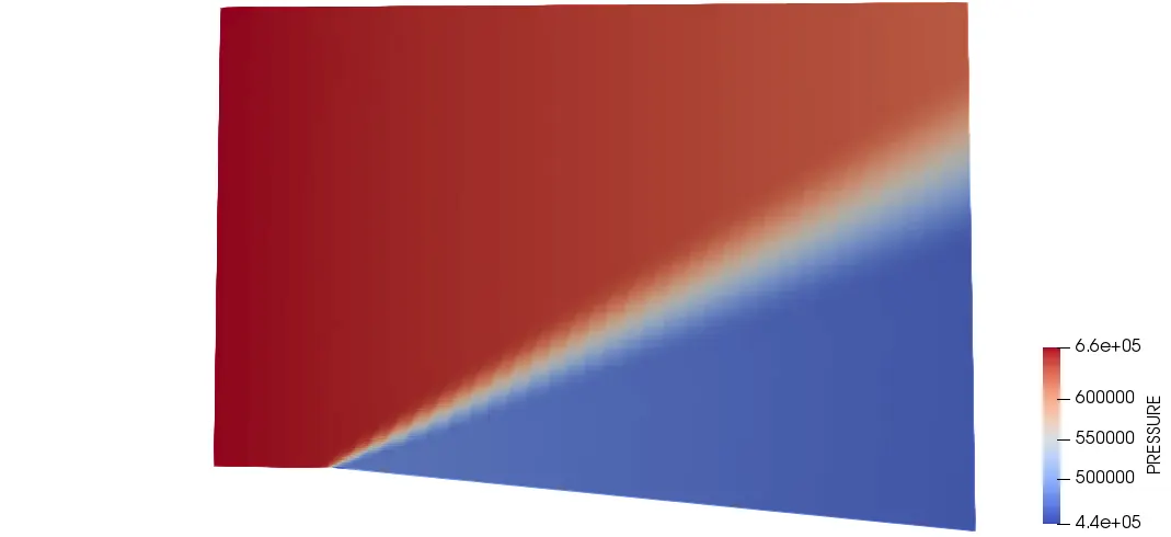
Case Study 2: Grid Size 0.8m SGS 0.01 Velocity 680m/s
Mesh Quality
Contour Plots
Velocity Contour
Pressure Contour
Temperature Contour
Line plots
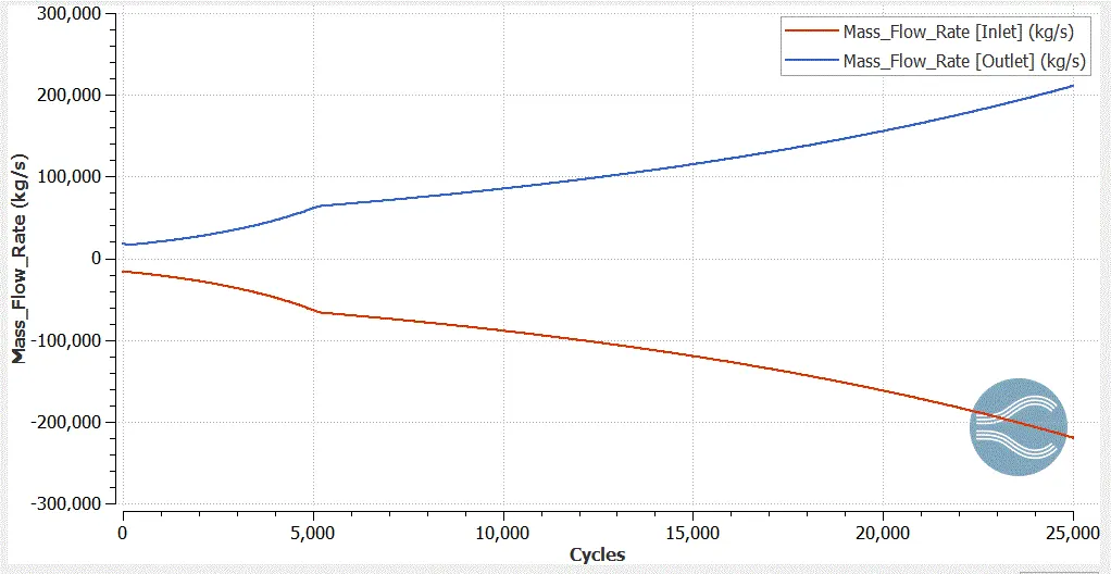
Mass Flow Rate
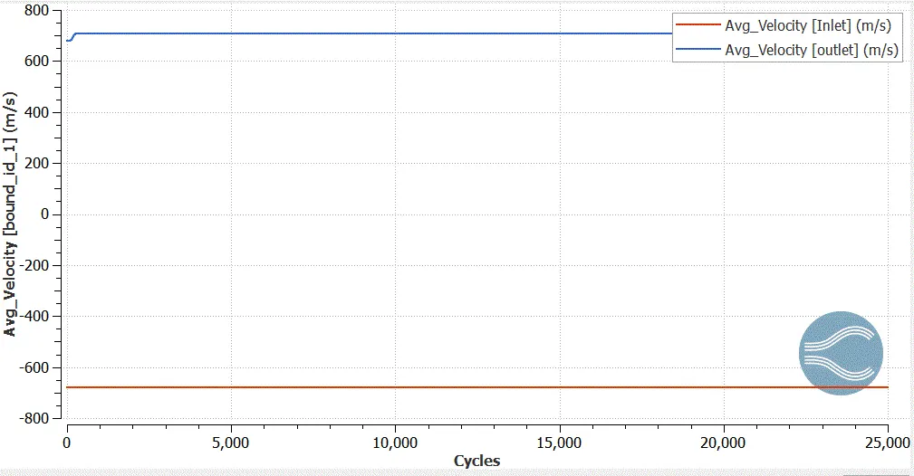
Velocity Plot
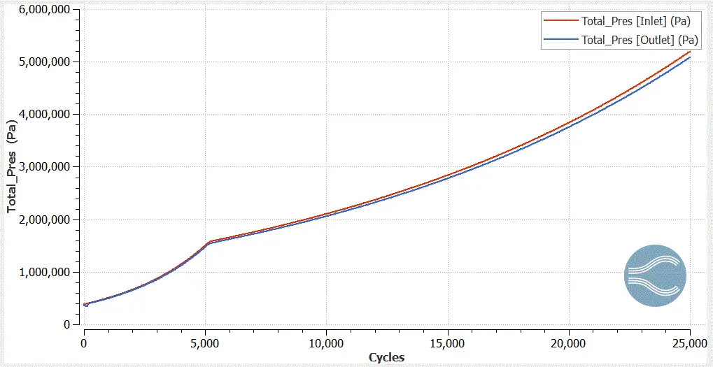
Pressure Plot
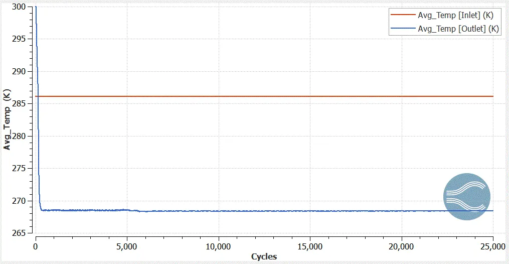
Temperature Plot
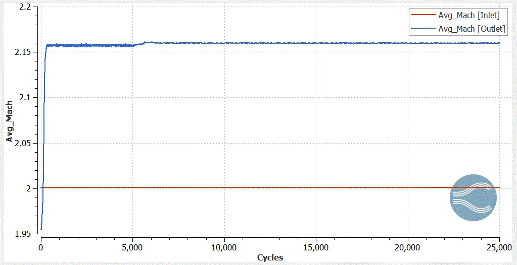
Mach Number Plot
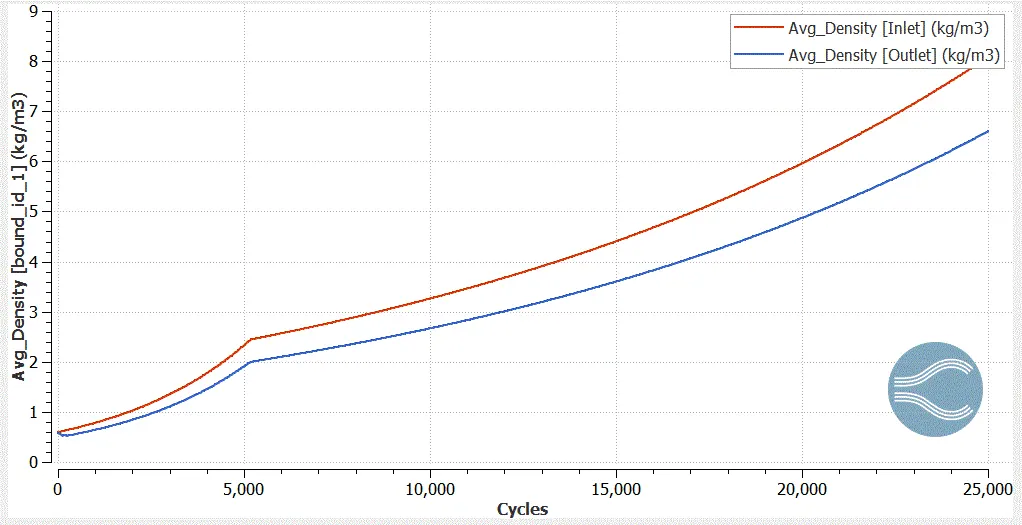
Density Plot
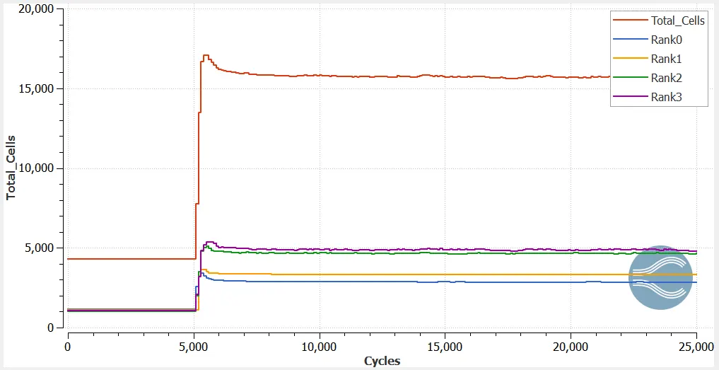
Cell Count
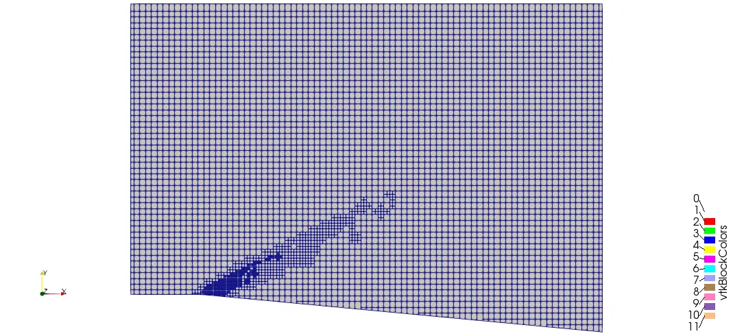
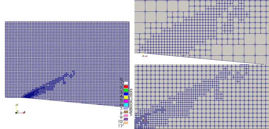
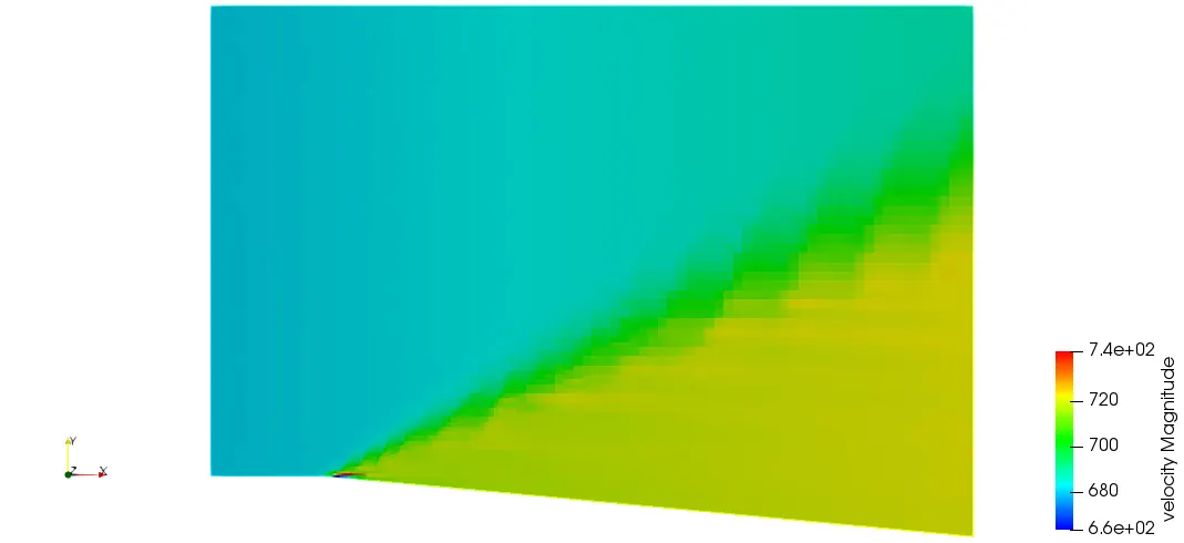
Case Study 3: Grid Size 0.8m SGS 0.1 Velocity 680m/s
Mesh Quality
Contour Plots
Velocity Contour
Pressure Contour
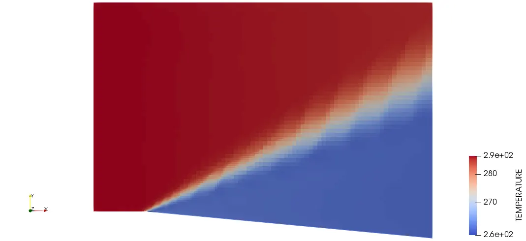
Temperature Contour
Line plots
Mass Flow Rate
Velocity Plot
Pressure Plot
Temperature Plot
Mach Number Plot
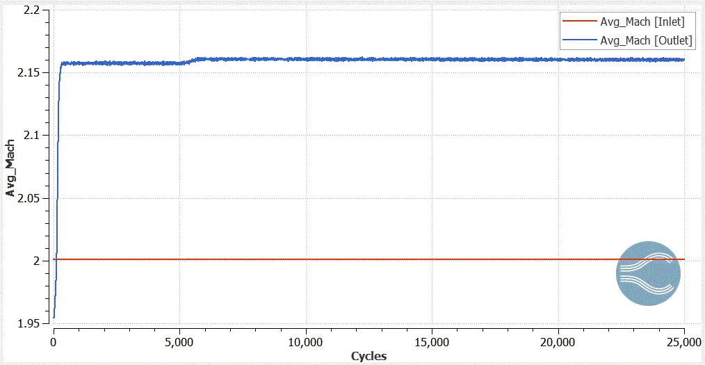
Density Plot
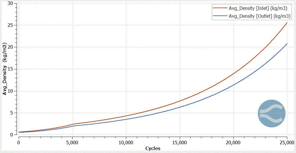
Cell Count
Subsonic Flow
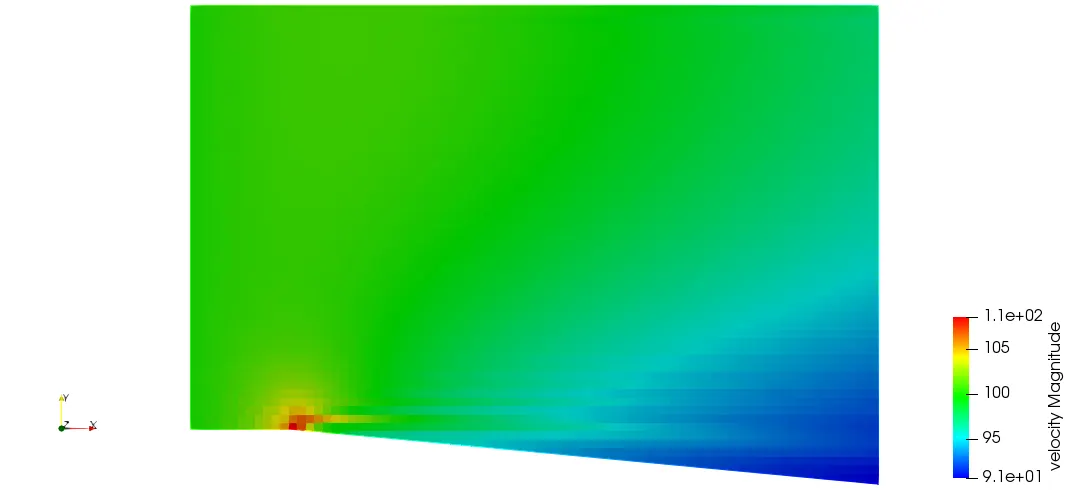
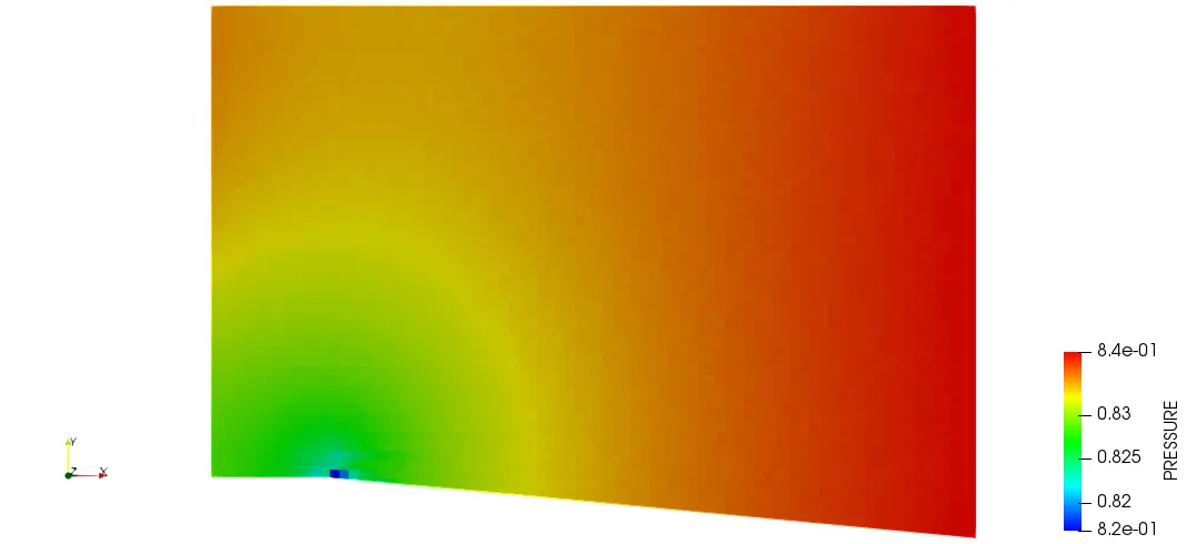
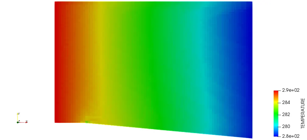
Case Study 4: Grid Size 0.8m SGS 0.05 Velocity 100m/s
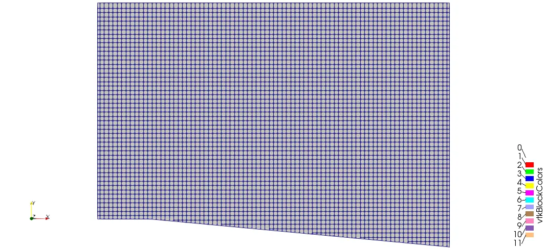
Mesh Quality
Contour Plots
Velocity Contour
Pressure Contour
Temperature Contour
Line plots
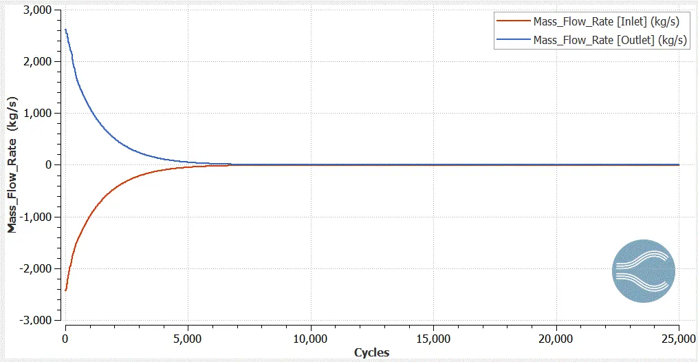
Mass Flow Rate
Velocity Plot
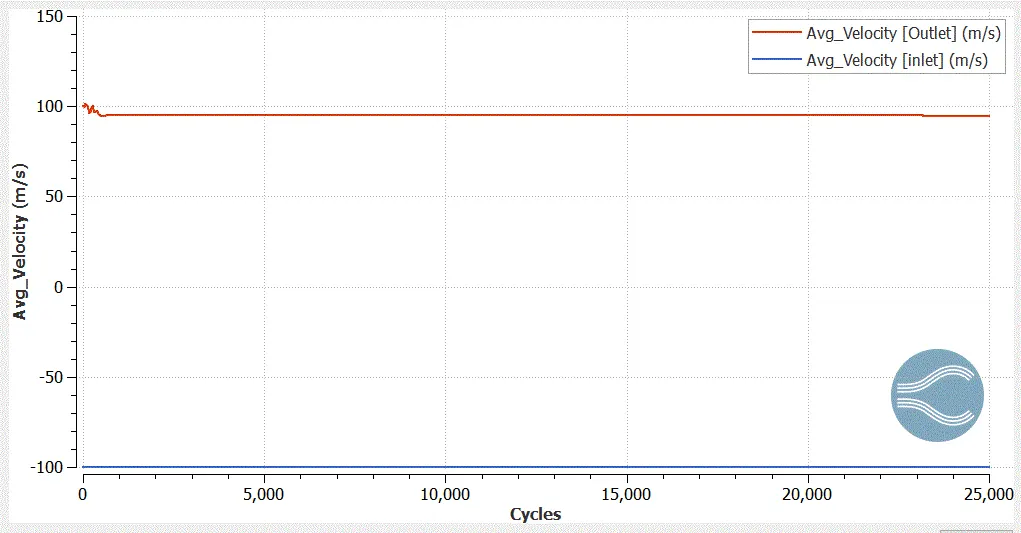
Pressure Plot
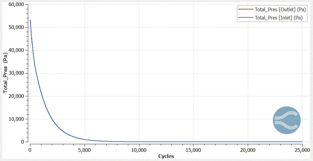
Temperature Plot
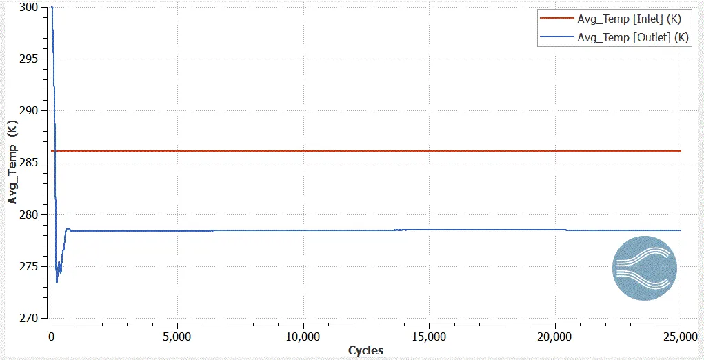
Mach Number Plot
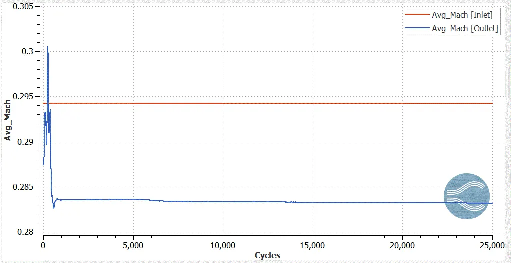
Density Plot
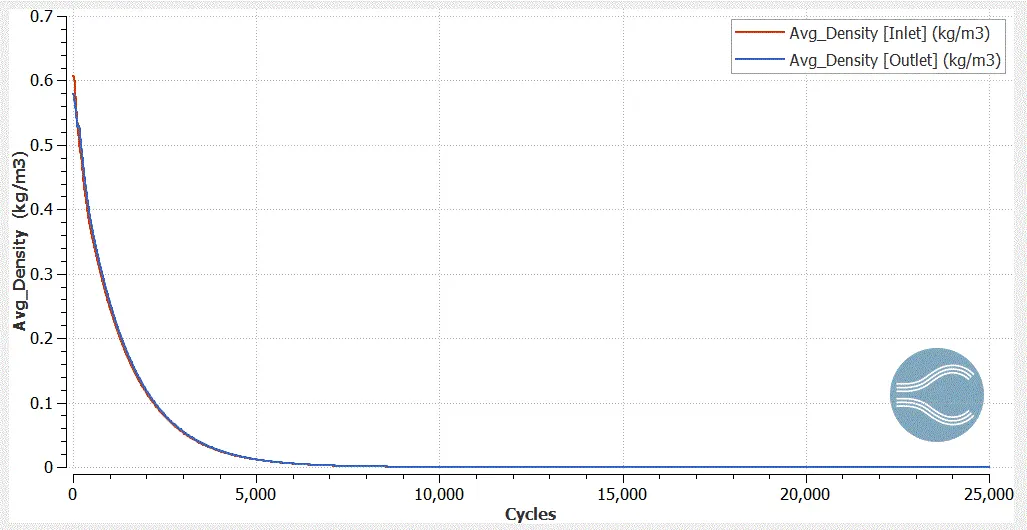
Cell Count
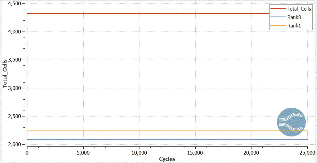
Conclusion
Many things can be noted when we change the value of SGS and inlet velocity.
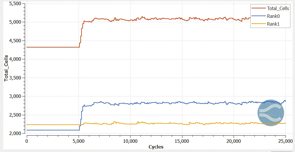
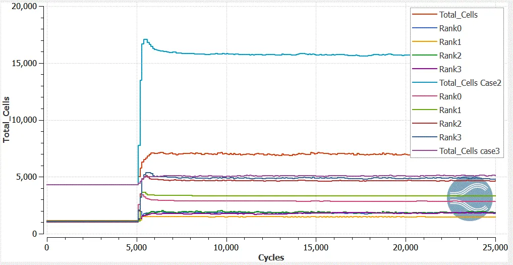
1. Cell count: Decrease in the SGS parameter, the cell count also increases to capture more data but the computational increses with increse in number of cells. can be seen from this plot.
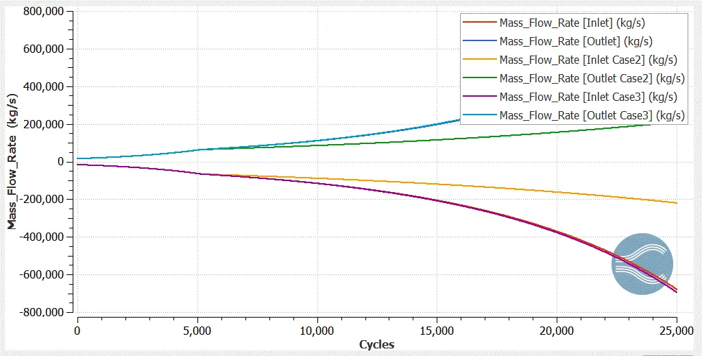
2.Mass Flow Rate: As the SGS decreases, There is increase in mass flow rate and can be compared using this plot.
3.Shock location: For the high SGS parameter, there is coarse quality mesh, and the smaller the value of SGS the mesh quality improves, Hence it affects the value of the case studies that can be seen in these plots.
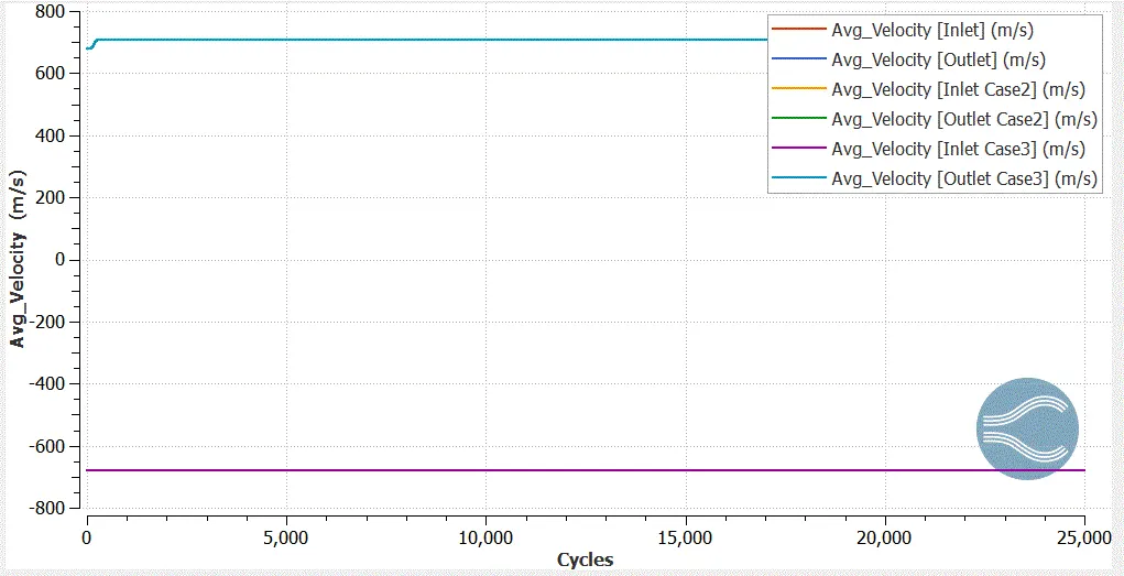
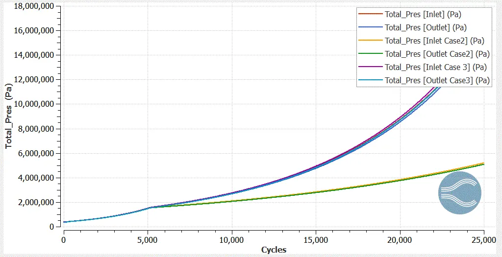
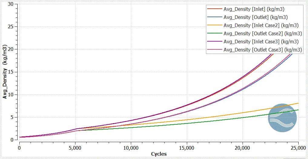
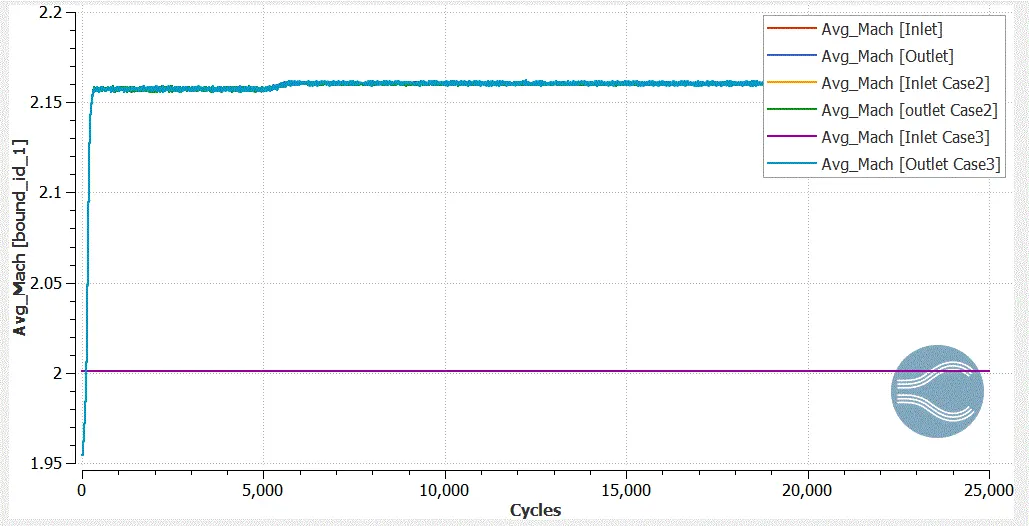
Supersonic V/S Subsonic Flow Comparision
in supersonic flow, as we already know that the match number of the flow is just twice a Prandtl-Meyer expansion fan can be seen near to sharp corner which is responsible for generating the shock waves and this area can we improved by reducing the value of SGS parameter in order to capture more cells.
Whereas on the other hand, in subsonic flow, there is not the formation of shock waves even after changing the SGS factor so at last, it can be concluded that the Prandtl-Meyer expansion fan occurs when the speed of flow is more than the speed of sound ie. 340m/s
The Case Study can be download from here case setup