Solving Second-Order Derivative Using Taylor Table in Matlab

Aim

The Major objective of the project was to create a program in Matlab to evaluate the second-order derivative of the analytical function `exp(x)*Cos(x)` and compare it with the 3 numerical approximations that you have been derived.

Introduction

Taylor Table is a type of table which contains the data of all the Taylor series expansion of a function that can be used to calculate the Analytical value of the higher-order derivative and pays an important role during Numerical discretization. The more the terms we include, we are closer to the accurate results.

If the Numerical Stencils are not symmetric then we call that as Skewed 2nd order scheme

Let us suppose we want `4^(th)` Order Accurate Approximation`

`frac{del^2f}{delx^2}` we need information at `i, i+1,i+2,i+3,i+4`

Skewed Right-Sided Difference

`frac{del^2f}{delx^2}=afunderset{i}{}+bfunderset{i+1}{}+cfunderset{i+2}{}+dfunderset{i+3}{}+efunderset{i+4}{}`

To solve this Expansion and Include all the data in Taylor Table

`afunderset{i}{}=afunderset{i}{}`

`b{funderset{i+1}{}}=b{funderset{i}{}+frac{Deltax}{1!}f'underset{i}{}+frac{Deltax^2}{2!}f''underset{i}{}+frac{Deltax^3}{3!}f'''underset{i}{}+frac{Deltax^4}{4!}f'''underset{i}{}}`

`c{funderset{i+2}{}}=c{funderset{i}{}+frac{2Deltax}{1!}f'underset{i}{}+frac{(2Deltax)^2}{2!}f''underset{i}{}+frac{(2Deltax)^3}{3!}f'''underset{i}{}+frac{(2Deltax)^4}{4!}f''''underset{i}{}}`

`d{funderset{i+3}{}}=d{funderset{i}{}+frac{3Deltax}{1!}f'underset{i}{}+frac{(3Deltax)^2}{2!}f''underset{i}{}+frac{(3Deltax)^3}{3!}f'''underset{i}{}+frac{(3Deltax)^4}{4!}f''''underset{i}{}}`

`e{funderset{i+4}{}}=e{funderset{i}{}+frac{4Deltax}{1!}f'underset{i}{}+frac{(4Deltax)^2}{2!}f''underset{i}{}+frac{(4Deltax)^3}{3!}f'''underset{i}{}+frac{(4Deltax)^4}{4!}f''''underset{i}{}}`

Taylor Table

Term	`f(x)`	`Deltaxf'(x)`	`Deltax^2f''(x)`	`Deltax^3f'''(x)`	`Deltax^4f''''(x)`
af(i)	a	0	0	0	0
bf(i+1)	b	b	b/2	b/6	b/24
cf(i+2)	c	2c	4c/2	8c/6	16c/24
df(i+3)	d	3d	9d/2	27d/6	81/24
ef(i+4)	e	4e	16e/2	64e/6	256e/24
`sum`	0	0	1	0	0

Its very important to find the Value of a,b,c,d,e in order to solve we use Matlab code

clear all
close all
clc

[A]=[1 1 1 1 1;0 1 2 3 4;0 1/2 2 9/2 8;0 1/6 4/3 9/2 32/3;0 1/24 2/3 27/8 32/3];
[B]=[0;0;1;0;0];

X=linsolve(A,B);
disp(X)

X=[2.916666666666668;-8.666666666666675;9.500000000000012;-4.666666666666674;0.916666666666668]

Skewed Left-Sided Difference

`frac{del^2f}{delx^2}=afunderset{i}{}+bfunderset{i-1}{}+cfunderset{i-2}{}+dfunderset{i-3}{}+efunderset{i-4}{}`

To solve this Expansion and Include all the data in Taylor Table

`afunderset{i}{}=afunderset{i}{}`

`b{funderset{i-1}{}}=b{funderset{i}{}-frac{Deltax}{1!}f'underset{i}{}+frac{Deltax^2}{2!}f''underset{i}{}-frac{Deltax^3}{3!}f'''underset{i}{}+frac{Deltax^4}{4!}f'''underset{i}{}}`

`c{funderset{i-2}{}}=c{funderset{i}{}-frac{2Deltax}{1!}f'underset{i}{}+frac{(2Deltax)^2}{2!}f''underset{i}{}-frac{(2Deltax)^3}{3!}f'''underset{i}{}+frac{(2Deltax)^4}{4!}f''''underset{i}{}}`

`d{funderset{i-3}{}}=d{funderset{i}{}-frac{3Deltax}{1!}f'underset{i}{}+frac{(3Deltax)^2}{2!}f''underset{i}{}-frac{(3Deltax)^3}{3!}f'''underset{i}{}+frac{(3Deltax)^4}{4!}f''''underset{i}{}}`

`e{funderset{i-4}{}}=e{funderset{i}{}-frac{4Deltax}{1!}f'underset{i}{}+frac{(4Deltax)^2}{2!}f''underset{i}{}-frac{(4Deltax)^3}{3!}f'''underset{i}{}+frac{(4Deltax)^4}{4!}f''''underset{i}{}}`

Taylor Table

Term	`f(x)`	`Deltaxf'(x)`	`Deltax^2f''(x)`	`Deltax^3f'''(x)`	`Deltax^4f''''(x)`
af(i)	a	0	0	0	0
bf(i-1)	b	-b	b/2	-b/6	b/24
cf(i-2)	c	-2c	4c/2	-8c/6	16c/24
df(i-3)	d	-3d	9d/2	-27d/6	81/24
ef(i-4)	e	-4e	16e/2	-64e/6	256e/24
`sum`	0	0	1	0	0

Its very important to find the Value of a,b,c,d,e in order to solve we use Matlab code

clear all
close all
clc

[A]=[1 1 1 1 1;0 -1 -2 -3 -4;0 1/2 2 9/2 8;0 -1/6 -4/3 -9/2 -32/3;0 1/24 2/3 27/8 32/3];
[B]=[0;0;1;0;0];

X=linsolve(A,B);
disp(X)

X=[2.916666666666668;-8.666666666666675;9.500000000000012;-4.666666666666674;0.916666666666668]

Central Differnce Scheme

`frac{del^2f}{delx^2}=afunderset{i-2}{}+bfunderset{i-1}{}+cfunderset{i}{}+dfunderset{i+1}{}+efunderset{i+2}{}`

`a{funderset{i-2}{}}=a{funderset{i}{}-frac{2Deltax}{1!}f'underset{i}{}+frac{(2Deltax)^2}{2!}f''underset{i}{}-frac{(2Deltax)^3}{3!}f'''underset{i}{}+frac{(2Deltax)^4}{4!}f''''underset{i}{}}`

`{funderset{i-1}{}}=b{funderset{i}{}-frac{Deltax}{1!}f'underset{i}{}+frac{Deltax^2}{2!}f''underset{i}{}-frac{Deltax^3}{3!}f'''underset{i}{}+frac{Deltax^4}{4!}f'''underset{i}{}`

`cfunderset{i}{}=cfunderset{i}{}`

`d{funderset{i+1}{}}=d{funderset{i}{}+frac{Deltax}{1!}f'underset{i}{}+frac{Deltax^2}{2!}f''underset{i}{}+frac{Deltax^3}{3!}f'''underset{i}{}+frac{Deltax^4}{4!}f'''underset{i}{}}`

`e{funderset{i+2}{}}=e{funderset{i}{}+frac{2Deltax}{1!}f'underset{i}{}+frac{(2Deltax)^2}{2!}f''underset{i}{}+frac{(2Deltax)^3}{3!}f'''underset{i}{}+frac{(2Deltax)^4}{4!}f''''underset{i}{}}`

Taylor Table

Term	`f(x)`	`Deltaxf'(x)`	`Deltax^2f''(x)`	`Deltax^3f'''(x)`	`Deltax^4f''''(x)`
af(i-2)	a	-2a	4a/2	-8a/6	16a/24
bf(i-1)	b	-b	b/2	-b/6	b/24
cf(i)	c	0	0	0	0
df(i+1)	d	d	d/2	d/6	d/24
ef(i+2)	e	2e	4e/2	8e/6	16e/24
`sum`	0	0	1	0	0

Its very important to find the Value of a,b,c,d,e in order to solve we use Matlab code

clear all
close all
clc

[A]=[1 1 1 1 1;-2 -1 0 1 2;2 1/2 0 1/2 2;-8/6 -1/6 0 1/6 8/6;16/24 1/24 0 1/24 16/24];
[B]=[0;0;1;0;0];

X=linsolve(A,B);
disp(X)

X=[-0.083333333333334;1.333333333333334;-2.500000000000001;1.333333333333334;-0.083333333333334]

Matlab Code to evaluate the second-order derivative of the analytical function exp(x)*cos(x)

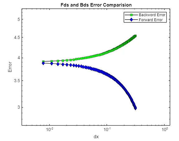
Code to Generate the error at different value of Forward Deri Scheme and Backward Deri Scheme compared with Analytical Deri

clear all
close all
clc

%taylor Table test
%analytical function f'=exp(x)*cos(x)
%f''=-2exp(x)*sin(x)

x=pi/3;
dx=linspace(pi/10,pi/400,100);
analytical_function=exp(x)*cos(x);
analytical_der=-2*exp(x)*sin(x);

for i=1:length(dx);
    bd(i)=(exp(x)*cos(x)-exp(x-dx(i))*cos(x-dx(i)))/dx(i);
    fd(i)=(exp(x+dx(i))*cos(x+dx(i))-exp(x)*cos(x))/dx(i);
    br(i)=abs(bd(i)-analytical_der);
    fr(i)=abs(fd(i)-analytical_der);
end

figure(1)
loglog(dx,br,'-ks','markerfacecolor','g')
hold on
loglog(dx,fr,'-kd','markerfacecolor','b')
hold on
legend('Backword Error','Forward Error')
xlabel('dx')
ylabel('Error')
title('Fds and Bds Error Comparision')

Function to Find Absolute Error Between Analytical and Skewed Difference Right

function error_SR = skewed_right_difference(x,dx)
 % Given function 
 %f(x) = exp(x)*cos(x)
 % second order derivative of the function
 second_order_derivative = -2*exp(x)*sin(x);
 % calculating skewed right difference value 
 skewed_right_difference = (((2.9166)*(exp(x))*(cos(x)))+((-8.666)*(exp(x+(1*dx)))*cos(x+(1*dx)))+((9.5)*(exp(x+(2*dx)))*cos(x+(2*dx)))+((-4.666)*(exp(x+(3*dx)))*cos(x+(3*dx)))+((0.9166)*(exp(x+(4*dx)))*cos(x+(4*dx))))/(dx^2);
 
 %Error calculation 
 error_SR = abs(second_order_derivative - skewed_right_difference);
end

Function to Find Absolute Error Between Analytical and Skewed Difference Left

function error_SL = skewed_left_difference(x,dx)
 
 % Given function 
 %f(x) = exp(x)*cos(x)
 % second order derivative of the function
 second_order_derivative = -2*exp(x)*sin(x);
 
 % Calculating the skewed left difference value 
 skewed_left_difference = (((2.9166)*(exp(x))*(cos(x)))+((-8.666)*(exp(x-(1*dx)))*cos(x-(1*dx)))+((9.5)*(exp(x-(2*dx)))*cos(x-(2*dx)))+((-4.666)*(exp(x-(3*dx)))*cos(x-(3*dx)))+((0.9166)*(exp(x-(4*dx)))*cos(x-(4*dx))))/(dx^2);
 %Error calculation 
 error_SL = abs(second_order_derivative - skewed_left_difference);
end

Function to Find Absolute Error Between Analytical and Central Difference

function error_CD = central_difference(x,dx)
 
 % Given function 
 %f(x) = exp(x)*cos(x)
 % Second order derivative of the function
 second_order_derivative = -2*exp(x)*sin(x);
 
 % Calculating the central difference value 
 central_difference = ((-0.0833)*(exp(x-(2*dx))*cos(x-(2*dx)))+(1.3333)*(exp(x-(1*dx))*cos(x-(1*dx)))+(-2.50000)*(exp(x)*cos(x))+(1.3333)*(exp(x+(1*dx))*cos(x+(1*dx)))+(-0.08333)*(exp(x+(2*dx))*cos(x+(2*dx))))/(dx^2); 
 %Error calculation 
 error_CD = abs(second_order_derivative - central_difference);
end

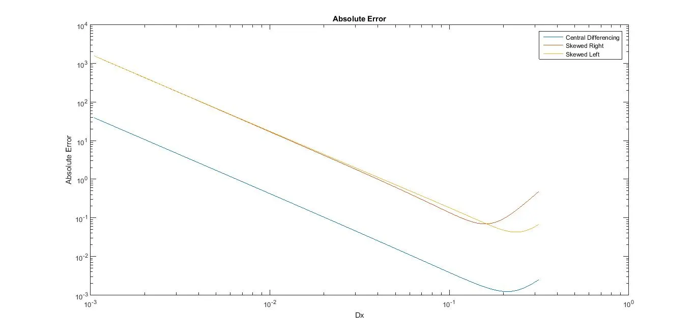
The main program that Calls all the three functions

close all
clc
% Input variables
x = pi/3;
dx = linspace(pi/10,pi/3000,200);
for i = 1:length(dx)
 central_diff_value(i) = central_difference(x,dx(i)); 
 skewed_right_value(i) = skewed_right_difference(x,dx(i));
 skewed_left_value(i) = skewed_left_difference(x,dx(i));
end
figure(1)
loglog(dx,central_diff_value)
hold on
loglog(dx,skewed_right_value)
loglog(dx,skewed_left_value)
hold off
title('Absolute Error')
legend('Central Differencing','Skewed Right','Skewed Left');
xlabel('Dx')
ylabel('Absolute Error')

Explanation

The major idea of this project was to find the absolute error between Analytical Solution and other solution that is Central diff, Skewed Left & Right Solution. Three functions were created and those functions were called using the main program in order to store a list of various values when we discretize on the basis of dx. Then the Log-log plot was plotted in Matlab.

Conclusion

At last, it can be concluded that the Central Differencing method has less error and we are more close to the more accurate results because it calculates the value from both sides, whereas if we talk about the Skewed Differencing Scheme Solution the error is little more its because the values are calculated on either left or right side for Skewed left and Skewed right respectively.

So Central Differencing Scheme is the best way to solve the solution of a function that provides more accuracy with less amount error.