Moving Reference Frame (MRF) project for fan modeling techniques

Problem Description:

An Icepak 3D fan object may sometimes behave differently from real fan behavior. Typically this is due to flow features like swirl and centrifugal spread resultant from the spinning fan rotor as well as the rotor blade geometry. In an Icepak fan-based setup, this swirl is estimated and calculated off a 2D annular flow face rather than off the physical surfaces of the blade.

The MRF approach allows for a more accurate representation of the internal geometry of the fan and therefore results in better modeling of the flow features. In Icepak MRF simulations, the actual blade geometry is modeled as a CAD block object and a fluid cylinder rotates into contact with the surfaces to create a spinning flow.

In this challenge, you will use a previously built Icepak model of fan blades and create the rotating MRF fluid blocks to create flow in the model. You will learn the proper problem setup and solution settings for an MRF model, as well as a good meshing technique to ensure good results. The Project file will be available below the respective video.

Objective:

The main objective of this project is to provide analysis and standards for the MRF fan modeling techniques for Moving Reference Frames(MRF) in ANSYS Icepak for the given CAD model.

Introduction for the Moving Reference Frame (MRF):

A Moving Reference Frame (MRF) is a relatively simple, robust, and efficient steady-state, Computational Fluid Dynamics (CFD) modeling technique to simulate rotating machinery. For example, the rotors on a quadcopter can be modeled with MRFs.

An MRF assumes that an assigned volume has a constant speed of rotation and the non-wall boundaries are surfaces of revolution (e.g., cylindrical, spherical, conical). In the case of the quadcopter example, the volumes between the rotor blades are designated as MRFs, assigned rotational speeds, and embedded within the multi-volume flow domain.

MRF is equivalent to running a rotational simulation and then observing the results at the instant equivalent to the position of the rotor within the MRF. MRF assumes a weak interaction between the MRF volume and the surrounding stationary volumes.

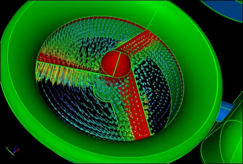
MRF CFD Simulation of Ducted Fan Shows velocity vectors within MRF volumes.

An alternative to MRF is the moving/sliding mesh technique, which can deal with strong interactions between the moving volume and the surrounding stationary volumes. However, in practice, the moving mesh technique often has robustness problems due to its dependence on intersection calculations between the stationary and rotating volumes. Also, the moving mesh technique is a transient (unsteady) simulation procedure which typically results in extremely long runtimes. Given the significant drawbacks of the moving mesh technique, the MRF is the preferred approach within its limitations.

Limitations for the MRF model:

Translation and rotational velocities are assumed to be constant (it is not allowed to vary in time.)

The specification of the relative velocity can not be used in conjunction with the MRF and mixture models. The absolute velocity definition is used instead for these situations. You don't need to have a single interface between reference frames where part of the interface consists of a two-sided coupled wall, while another part is not coupled. (i.e the normal interface treatment).

In such cases, the interface must be broken down into two interfaces: This is a coupled interface and the other is a fluid-fluid regular interface.

Geometry:

The cabinet is created with a 730mm*12mm*180 mm dimension, and the proper CAD model is installed in the cabinet.

We replaced them with the grilles for the air intake and exhaust instead of the vents for the CAD model.

The fan model provided by the default Icepak is not used here

A Resistance type of perforated thin vent resistance is used with 465741 of the free area ratio. The CAD model imported it looked like as

Meshing:

We have toggled the mesh assemblies separately in the mesh control to obtain the non-conformal networking.

A non-conformal network, whether the nodes at the device suit slightly or none. That means that, on one side of the interface, one, few, or every node has no match on the other. Calculations for non-conformal interfaces are done using a simulated polygon system that stores the vector and centroid areas of the polygon faces.

There is no movement in the node and cells are not necessarily waterproof cells. The gradients are therefore adjusted to take the missing face area into account.

Here we have generated a non-conformal mesh with the number of elements are 1118746 and the number of nodes is 1217943.

Slack values can be defined in such a way that the cells on each side of the interface are either fluid or rigid, of the same content, and should not break any of the "Non-Conformal Assembly Laws" set out in the connection. A slack value of 3 and 5 mm is used for the assemblies.

Here the max element size is taken as 4 which is the element is divided into 2 by 2 first then 1 by 1 and finally 0.5 and 0.5 after anyway.

Multi-level options help capture objects of various scales with lower mesh count.

Here the max level is given as it is 3 for the fan blades and the applied level is 2 for all components except for fan cases.

The meshing for the CAD model in X-axis looked like:

In this picture, we can see the non-conform mesh is formed and, at the same time, the elements in the mesh are closely attached for the fan blades ae which is a necessary parameter.

This is a display of fan blades model mesh shows show the meshing elements are plotted over the blades.

The Mesh in Y-axis looks like

The Mesh in Z-axis looks like

Numerical settings:

Basic parameters:

In the Basic parameters, we have considered the flow, and radiation was turned on and the flow region was considered to be Turbulent as the Realizable two-equation.

In this, we are solving both the flow and temperature variables for the CAD model given. We are neglecting the radiation effects because we are interested in solving the moving Reference Frame model (MRF) model.

Here in the fluid part in the CAD model which consists of the blades we have to give the MRF rotation. We need to give the rotational speed of 6000 RPM for the MRF.

Basic settings:

Here in the basic settings panel, we need to give the number of iterations to 1000. The convergence criteria for the flow is 1e-5, and for energy, turbulent kinetic energy and dissipation rate the criteria is 1ed-7.

From the residual map, we have shown that nearly at the iteration no.700 the solution converges. This can be understood by seeing the temperature and velocity control points set. The solution remains the same after iteration no 700, and we do not observe any instability in the residual plot.

At the same time, the continuity of velocity and the equation of energy is far below the ranges which we used in the simple setting of iterations. All that implies is that the solutions converge very well.

The disturbances in the epsilon curve reflect the swirl and turbulence phenomenon within the CAD model, as we set the fan rotation to 6000 rpm and the grille's free air ratio is 0.4 million.

Temperature Monitor points:

Here we can see that the solution remains constant and unchanged after the iterations number 700. the max temperature recorded is nearly 48 degrees centigrade and the least is 0.

Velocity Monitor points:

Here in the monitor points plot, we have seen that the velocity at the monitor points we set remains unchanged after the 700 iterations. The max velocity recorded is 21m/sec inside the CAD model but there in monitor points, it is below 8 m/sec because it shows the velocity only at the monitor points.

Parallel settings:

Here we have to use the parallel option and given the six processors because my PC supports till this point. We can increase or decrease the number of processors as per they are suitable in the PC.

Advanced solver setup:

In applied mathematics, discretization is the process of transferring continuous functions, models, variables, and equations into discrete counterparts. This process is usually carried out as a first step toward making them suitable for numerical evaluation and implementation on digital computers.

The discretization scheme properties were set accordingly as shown below

Examine and post-process the results:

Temperature :

The temperature contour was set to position accordingly to the z plane through the plane and it is clearly seen that the initial temperature for the opening side was at the 19.9°C and a maximum temperature of 47.3°C was obtained in the domain and the temperature inside the solid domain was nearly at 56.43°C.

Animation for the Temperature profile on the Cut plane in the Z-axis:

The Temperature animation which represents the temperature magnitude over the MFR model surface was shown in the above animation.

Velocity contour:

The Velocity Contour was set to position accordingly to the Z-plane through the plane and it is clearly seen that the initial velocity for the opening was at the initial value of 2.69m/sec and a maximum velocity was at the value of 21.43 m/sec was obtained in the domain and the velocity inside the domain was nearly at 13.39 m/sec.

Animation for the Velocity contour profile on the Cut plane in the Z-axis:

The Velocity animation which represents the Velocity contour over the MFR model surface was shown in the above animation.

Pressure contour:

The Pressure Contour was set to position accordingly to the x-plane through the plane and it is clearly seen that the initial pressure for the opening was at the initial value of 6.36N/m^2 and a maximum pressure was at the value of 107.08 N/m^2 was obtained in the domain and the pressure inside the domain was nearly at 39.93 N/m^2.

Animation for the Pressure profile on the Cut plane in the Z-axis:

The Pressure animation which represents the pressure contour over the MFR model surface was shown in the above animation.

Vector Contour:

The Velocity Contour was set to position accordingly to the Z-plane through the plane and it is clearly seen that the initial velocity for the opening was at the initial value of 2.69m/sec and a maximum velocity was at the value of 21.43 m/sec was obtained in the domain and the velocity inside the domain was nearly at 13.39 m/sec.

Animation for the Velocity vectors contour profile on the Cut plane in the Z-axis:

The Velocity vector animation which represents the Velocity contour over the MFR model surface was shown in the above animation.

Stream particles profile:

A streamline is a path traced out by a massless particle as it moves with the flow. It is easiest to visualize a streamline. The stream-lines profile was shown below on the total domain in the MRF.

Conclusion:

Modeling the Moving Reference Frame(MRF) allows for more accurate flow predictions. MRF reduces errors in predicting the temperature of components because it throws the flow directly onto the components. We can't get through this phenomenon with the usual fan modeling.

MRF modeling is very precise in predicting flow, turbulence, and noise levels in the system. This model also gives accurate results of flow, temperature, and some other parameters even in high-density electronic models.