Week 4 - Genetic Algorithm

AIM:

To calculate the global maxima of a stalagmite function in MATLAB.

Objective:
To write a code in MATLAB to optimize the stalagmite function and find the global maxima of the function.

To plot graphs for all 3 studies and for F maximum vs no.of iterations.

Theory:

Genetic Algorithm is a search based optimization technique based on the principle of Genetics and Natural Selection. It is frequently used to find optimal or near-optimal solutions to difficult problems that otherwise would take a lifetime to solve. It is frequently used to solve optimization problems in research and in machine learning.

Nature has always been a great source of inspiration to all mankind Genetic Algorithms (GAs) are search based algorithms based on the concepts of natural selection and genetics.GAs are a subset of a much larger branch of computation known as Evolutionary Computation.

A genetic algorithm is a search heuristic that is inspired by Charles Darwin's theory of natural evaluation. This algorithm reflects the process of natural selection where the fittest individuals are selected for reproduction in order to produce offspring of the next generation.GAs was developed by John Holland and his students and colleagues at the University of Michigan, most notably David E. Goldberg, and has since been tried on various optimization problems with a higher degree of success.

In GAs, we have pooled a population of possible solutions to the given problem. These solutions then undergo recombination and mutation like in natural genetics producing new children and the process is repeated over various generations. Each individual is assigned a fitness value based on its objective function values and the fitter individuals are given a higher chance to mate and yield more fitter individuals. This is in line with the Darwinian Theory of "Survival of the Fittest".In this way, we keep evolving better individuals or solutions over generations till we reach a stopping criterion.

Genetic algorithms are sufficiently randomized in nature but the perform much better than random local search in which we just try various random solutions keeping track of the best so far as they exploit historical information as well.

Advantages of GAs:

GAs have various advantages that have made them immensely popular. These include

• Does not require any derivative information which may not be available for many real-world problems.
• Is faster and more efficient as compared to the traditional methods
• Has very good parallel capabilities
• Optimizes both continuous and discrete functions and also multi-objective problems
• Provides a list of good solutions and not just a single solution
• Always get an answer to the problem which get better over the time
• Useful when the search space is very large and there are a large number of parameters involved.

Limitations of GAs:

Like any technique GAs also suffer from a few limitations these includes

• GAs are not suited for all problems especially problems that are simple and for which derivative information is available.
• The fitness value is calculated repeatedly which might be computationally expensive for some problems.
• Being stochastic there are no guarantees on the optimality or the quality of the solution.
• If not implemented properly the GA may not converge to the optimal solution.
• The genetic algorithm uses three main types of rules at each step to create the next generation from the current population.
• Selection rules select the individuals, called parents that contribute to the population at the next generation.
• Crossover rules combine two parents to from children for the next generation.
• Mutation rules apply random changes to individual parents to the form of children.
• The genetic algorithm differs from a classical derivative-based optimization algorithm in two main ways as summarized in the following tables.

Classical Algorithm	Genetic Algorithm
Generates a single point at each iteration. The sequence of points approaches optimal solutions	Generates a population of points at each iteration. The best point in the population approaches an optimal solution
Select the next point in the sequence by a deterministic computation	Select the next population by computation which uses the random number generators.

Governing Equations:

`f(x,y) =f_(1,x)*f_(2,x)*f_(1,y)*f_(2,y)`

`f_(1,x)=(sin(5.1pix+0.5))^6`

`f_(1,y)=(sin(5.1piy+0.5))^6`

`f_(2,x)=exp(-4ln(2)((x-0.0667)^2/(0.64)))`

`f_(2,x)=exp(-4ln(2)((y-0.0667)^2/(0.64)))`

Solution Steps:

1. The first two input variables x and y were created which were one-dimensional arrays of 150 equally spaced values between 0 and 0.6 using linspace command and then a two-dimensional matrix of these variables was created using mesh grid command.
2. Another function named stalagmite was created separately which stores the two input variables and contains equations for outputs and was called in the main program
3. The results from the stalagmite function were stored in another variable(F) and plotted as a surface using the surface command in MATLAB.
4. ''ga'' function was used to calculate the maximum values of stalagmite function but since "ga" command gives minimum values of function provided so some changes had to be made to get desired resutls, so a '-' sign was used to before (f) to get maximum values from "ga" command.
5. Then our code was made to iterated 50 times using for loop t study the statistical behavior of genetic algorithm with unbounded inputs bounded inputs, bounded inputs with increasing populations and all these studies are plotted individually using subplot,plot3, and sufc command.
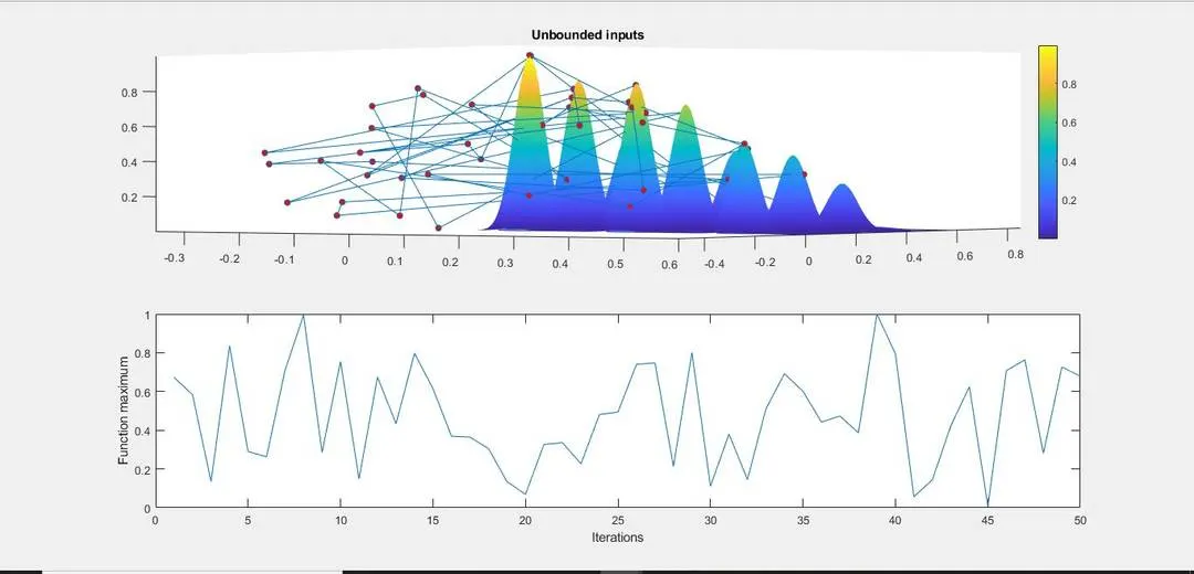
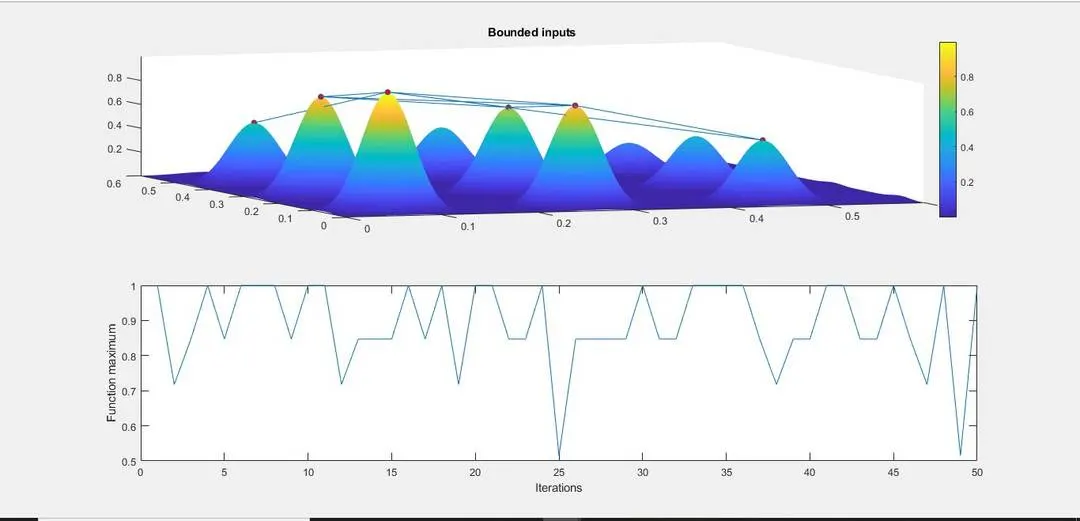
6. The results obtained from all three studies differ from each other as in the first study of unbounded inputs during each iteration the maximum values changes from 0 to 1 so in the second study of bounded inputs "ga" command is changed and the upper and lower bounds of 0 and 1 are set respectively in this case the results obtained are much sophisticated as compared to first one.
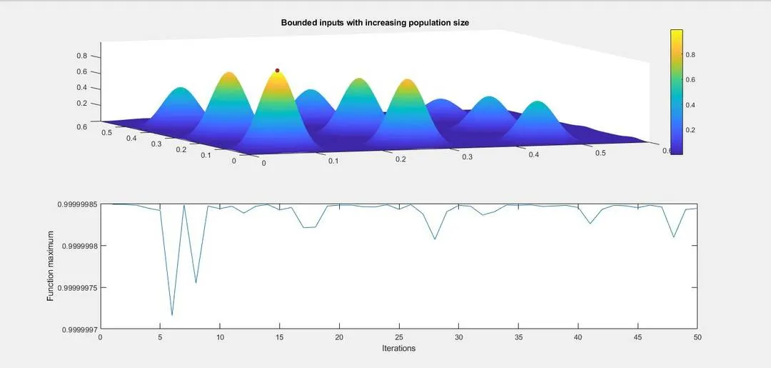
7. Hence in the third study of bounded inputs with increasing population size which was 50 by defaults, it was increased to 300. The output results obtained were confined to a very small range of 0.99 and it was approximately accurate resutls. If the population size was increased furthermore accurate results will be obtained.

Description of Syntax of "Ga"

x = ga(fun,nvars) find a local unconstrained minimum,X, to the objective function fun.nvars is the dimension(number of design variables) of fun.

x = ga(fun,nvars,A,b)finds a local minimum x to fun subject to the linear in equalities A*x <= b.
ga evaluates the matrix product A*x as if x is transposed(A*x’).

x=ga(fun,nvars,A,bA,eq,beq) find a local minimum x to fun, subject to the linear equalities Aeq*x=beq and A*x <= b . (Set A=[ ] and b=[ ] if no linear inequalities exist.) ga evaluates the matrix product Aeq*x as if x is transposed(Aeq*x’).

x=ga (fun,nvars,A,b,Aeq,beq,lb,ub) defines a set of lower an upper bounds on the design variables,x, so that a solution is found in the range lb <= x<= ub.(Set Aeq=[ ] and beq =[ ] if no linear equalities exist.)

x= ga(fun,nvars,A,b,Aeq,beq,lb,ub,nonlcon,options) minimize with the default optimization parameters replaced by values in options. (Set nonlcon=[ ] if no nonlinear constraints exists.)Create options using optimoptions.

x= ga(fun,nvars,A,b,[ ],[ ],Aeq,beq,lb,ub,nonlcon,IntCon) or x =ga(fun,nvars,A,b,[ ],[ ],lb,ub,nonlcon,Intcon,options) requires that the variables listed in IntCon take integer values.

MATLAB CODE:

Code containing stalagmite function:

function [f] = stalagmite(input_vector)

x = input_vector(1)
y = input_vector(2)

f_1_x = (sin(5.1*pi*x + 0.5))^6
f_1_y = (sin(5.1*pi*y + 0.5))^6
f_2_x = exp(-4*log(2)*((x-0.0667)^2/0.64))
f_2_y = exp(-4*log(2)*((y-0.0667)^2/0.64))
% Negative sign is used to return max values from ga command
[f] = -((f_1_x)*(f_2_x)*(f_1_y)*(f_2_y))

end

Main code containing the first study:

% A program t calculate the maxima of a function with unbounded inputs

clear all
close all
clc


%inputs for search space

x = linspace(0,0.6,150)
y = linspace(0,0.6,150)
num_cases = 50

%creating a 2_dimensional mesh

[xx,yy] = meshgrid(x,y)

%evaluting the stalagmite function

for i = 1:length(xx)
    for j = 1:length(yy)
        input_vector(1) = xx(i,j);
        input_vector(2) = yy(i,j);
        f(i,j) = stalagmite(input_vector);
    end
end

tic
%study-1-Statistical behaviour wiht unbounded input values

for a = 1:num_cases
    [inputs,fopt_1(a)] = ga(@stalagmite,2);
    xopt(a)=inputs(1);
    yopt(a)=inputs(2); 
end
study1_time=toc

%plotting our data

figure(1)
subplot(2,1,1)
hold on 
surfc(x,y,-f)
shading interp
colorbar
plot3(xopt,yopt,-fopt_1,'marker','o','markerfacecolor','r','markersize',5)
title('Unbounded inputs')
subplot(2,1,2)
plot(-fopt_1)
xlabel('Iterations')
ylabel('Function maximum')

Main code containing the Second study:

% A program t calculate the maxima of a function with unbounded inputs

clear all
close all
clc


%inputs for search space

x = linspace(0,0.6,150)
y = linspace(0,0.6,150)
num_cases = 50

%creating a 2_dimensional mesh

[xx,yy] = meshgrid(x,y)

%evaluting the stalagmite function

for i = 1:length(xx)
    for j = 1:length(yy)
        input_vector(1) = xx(i,j);
        input_vector(2) = yy(i,j);
        f(i,j) = stalagmite(input_vector);
    end
end

tic

%study-2-Statistical behaviour wiht upper and lower bounded input values

for b = 1:num_cases
    [inputs,fopt_2(b)] = ga(@stalagmite,2,[],[],[],[],[0;0],[1;1]);
    xopt(b)=inputs(1);
    yopt(b)=inputs(2);
    
end

study2_time=toc

%plotting our data

figure(2)
subplot(2,1,1)
hold on 
surfc(x,y,-f)
shading interp
colorbar
plot3(xopt,yopt,-fopt_2,'marker','o','markerfacecolor','r','markersize',5)
title('Bounded inputs')
subplot(2,1,2)
plot(-fopt_2)
xlabel('Iterations')
ylabel('Function maximum')

Main code containing the Third study:

% A program t calculate the maxima of a function with unbounded inputs

clear all
close all
clc


%inputs for search space

x = linspace(0,0.6,150)
y = linspace(0,0.6,150)
num_cases = 50

%creating a 2_dimensional mesh

[xx,yy] = meshgrid(x,y)

%evaluting the stalagmite function

for i = 1:length(xx)
    for j = 1:length(yy)
        input_vector(1) = xx(i,j);
        input_vector(2) = yy(i,j);
        f(i,j) = stalagmite(input_vector);
    end
end

%study-3-Statistical behaviour with upper and lower bounded input values and increasing genetic algorithm iterations

option_1 = optimoptions('ga')
option_1 = optimoptions(option_1,'Populationsize',300)

tic

for c = 1:num_cases
    [inputs,fopt_3(c)] = ga(@stalagmite,2,[],[],[],[],[0;0],[1;1],[],[],option_1);
    xopt(c)=inputs(1);
    yopt(c)=inputs(2);
    
end

study3_time=toc

%plotting our data

figure(3)
subplot(2,1,1)
hold on 
surfc(x,y,-f)
shading interp
colorbar
plot3(xopt,yopt,-fopt_3,'marker','o','markerfacecolor','r','markersize',5)
title('Bounded inputs with increasing population size')
subplot(2,1,2)
plot(-fopt_3)
xlabel('Iterations')
ylabel('Function maximum')

Results:

Study-1

Study-2

Study-3

Note: Genetic algorithm with different results at each run so use rng('default') to set the random number generator to a known value.

Errors and Remedies: The were no errors encountered except one mistake that I'd saved the main program under the same name as ga and it results in an error while solving so to rectify it the main program was renamed under the different file name.

Conclusion: The genetic algorithm repeatedly modifies a population of individual solutions. At each step, the genetic algorithm selects individuals at random from the current population to be parents and uses them to produces the children for the next generation. Over successive generations, the population "evolves" toward an optimal solution. But if the population size is taken too large the processing time taken by Matlab also increases.