Week 3 - Solving second order ODEs

Aim:

A program to simulate the transient behavior of a simple pendulum and to create an animation of its motion.

Sub-Objectives:

• Write a program to solve the ODE
• Plot the displacement v/s time and velocity v/s time graphs
• Create an animation of the motion of the pendulum

Introduction:

In Mathematics an ordinary differential equation is a differential equation containing one or more functions of one independent variable and the derivatives of those functions. The term ordinary is used in contrast with the term partial differential equation which may be with respect to more than one independent variable.

• A second-order ordinary differential equation is an ordinary differential equation in which any derivatives with respect to the independent variable have order no greater than 2''>2
• The ordinary differential equation helps us to solve the many engineering systems such as harmonic, vibrations, damping, etc.
• Second-order linear differential equations are used to model many systems in engineering.
• A simple pendulum consists of a mass "m" hanging from a string of length ''l'' and fixed at a pivoted point. when displaced to an initial angle 'θ' and released the pendulum will swing back to front with periodic motion

The equation is given by,

and some hand calculation for getting 2_order_ode into first order

We are going to use the 2nd order ODE equation to find out the velocity and position of the pendulum ball with respect to time.

g = gravity in m/s2,

L = length of the pendulum in m,

m = mass of the ball in kg,

b=damping coefficient.

Inputs are taken as given in the problem

L = 1meter

m= 1kg

b=0.05

g=9.81m/s^2

Initial conditions are taken as

Angular displacement =0;

Angular velocity=3 rad/sec,at time t=0;

the time motion given is between 0-20sec

Solving ODE:

ODE45 is usually the function of choice among the ODE solvers. It compares methods of orders four and five to estimate error and determine step size. ODE45 is so accurate that its default behavior is to use its interpolant to provide results at intermediate points.

Ode solver ode45 is used in this program. the results are stored in an array of row matrix of two columns for the values of displacement and velocity at different time periods

ode_function is the function made to solve the given equation where the assumption is made in the from the code

Code

ODE Function Program:

function [dtheta_dt] = ode_function(t,theta,b,g,l,m)

theta1 = theta(1);
theta2 = theta(2);


dtheta1_dt = theta2;
dtheta2_dt = -(b/m)*theta2 - (g/l)*sin(theta1)

dtheta_dt = [dtheta1_dt;dtheta2_dt];
end

Matlab program to simulate pendulum motion and creating animation:

%Program to solve the ODE and simulatethe pendulum motion

clear all
close all
clc

%Inputs
% damping coefficient value
b = 0.05;
%Gravitational value in m/s^2
g = 9.80;
%Length of the pendulum in m
l = 1;
%mass of the body in kg
m = 1;


%Initial condition for displacement and velocity
theta_0 = [0;3];

%Time span points
t_span = linspace(0,20,400);

%Solving ODE
[t,results] = ode45(@(t,theta) ode_function(t,theta,b,g,l,m),t_span,theta_0)

%Plotting
figure(1)
plot(t,results(:,1),'color','r')
hold on
grid on
plot(t,results(:,2),'color','g')
xlabel('Time')
ylabel('Plot')
legend('Displacement','Velocity')

figure(2)
plot(results(:,1),results(:,2))
xlabel('position-radian')
ylabel('angular velocity - radians/sec')
title('angular velocity')
legend('angular velocity')

figure(3)
ct = 1;
for i = 1:length(results(:,1));
    THETA_1 = results(i,1);
    % Initial co-ordinates
    x0 = 0;
    y0 = 0;
    
    x1 = 1*sin(THETA_1);
    y1 = -1*cos(THETA_1);
    
    %Plot
    plot([-0.5 0.5],[0,0],'color','c')
    line([x0 x1],[y0,y1],'color','b')
    hold on
    plot(x1,y1,'marker','o','markersize',25,'markerfacecolor','r')
    grid on 
    title('Moving Pendulum with function of time')
    axis ([-1.5 1.5 -1.5 1])
    hold off
    pause(0.001)
    M(ct) = getframe(gcf);
    ct = ct+1;    
end

movie(M)
videofile = VideoWriter('Second_ODE_Pendulum.avi','uncompressed AVI');
open(videofile)
writeVideo(videofile,M)
close(videofile)

To make videos in Matlab we have to write

• The graph is plotted using the plot command. The get frame(gcf) command is used inside the loop to get the current frame and store it as an image into the array 'M'.
• The video writer command creates an empty video file by the name 'Second_ODE_Pendulum' in.avi format and it is stored in the variable video file.
• The write video command inserts the frames stored in array 'M' into the video file

we have created an uncompressed file called forward kinematics.avi and assigning it to variables

movie(M)
videofile = VideoWriter('Second_ODE_Pendulum.avi','uncompressed AVI');
open(videofile)
writeVideo(videofile,M)
close(videofile)

Error and Reminders:

The above error was rectified by putting 'VideoWriter'

Error-2

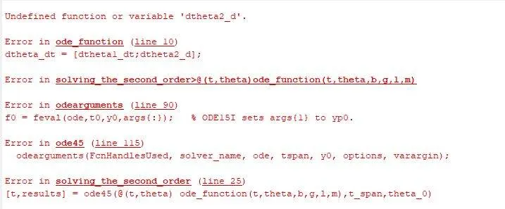
In the ode function, we have cleared this error by keeping the "dtheta2_dt"

Results:

The displacement v/s time and velocity v/s time graphs were plotted.

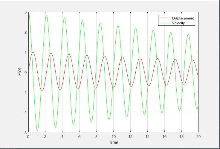
Here the graph is plotted to get the waveform of the displacement and the velocity from the initial condition and the change in the displacement and velocity has been noticed.

Angular velocity:

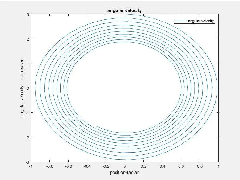
Angular velocity, also called rotational velocity, is a quantitative expression of the amount of rotation that a spinning object undergoes per unit of time. It is a vector quantity, consisting of an angular speed component and either of two defined directions.

Animation the Pendulum Motion:

Here we use the concepts of the 'For-loop' as the bob moves with velocity and displaces for the different time periods. And recorded it and animated the path of the oscillation.

The animation video for the pendulum motion was created using Matlab.