Gate Valve Parametric Study

Aim:-> To perform parametric study on gate valve simulation in ANSYS Fluent.

Theory:-

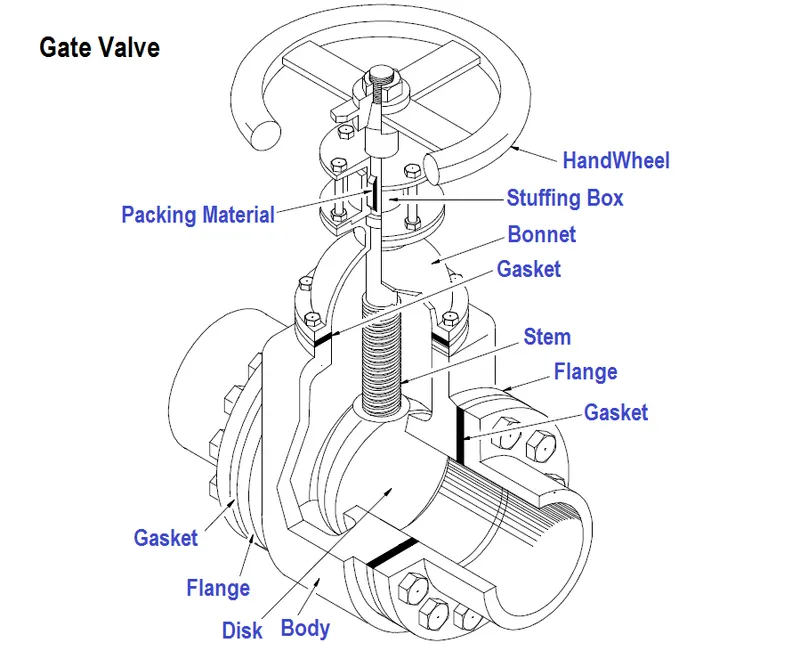Fig: Gate valve schematic diagram

As shown in above figure, gate valve's main components are body, seat, gate, stem, bonnet, and actuator.

The primary operation mechanism is straightforward. Turning the handwheel rotates the stem, which moves the gate up or down via the threads. They require more than one 360° turn to fully open/close the valve. Lifting the gate from the path of the flow, the valve opens. Lowering the gate to its closed position seals the bore resulting in a full closure of the valve.

For a gate valve, the relationship between the gate's vertical travel and the flow rate is nonlinear, with the highest changes occurring near shutoff. When used to regulate flow, the relatively high velocity of the flow at partial opening results in gate and seat wear, which along with possible vibrations of the gate, shortens the valve's service life.

Gate valve may be classified in following types:

1. Types of disc:

• Solid taper wedge
• Flexible wedge
• Split wedge or Parallel disks Valve

2. Types of Body Bonnet Joint

• Screwed Bonnet
• Bolted-Bonnet
• Welded-Bonnet
• Pressure-Seal Bonnet

3. Types of Stem movement

• Rising Stem or OS & Y Type (Outside Stem and Screw Type)
• Non-rising Stem type

Reynolds number (Re):

To find out Reynold number, we know that-

`Re=(rhoxxVxxL)/mu`

Where,

`rho=density=998.2(kg)/m^3`

`V="Inlet velocity"=0.1415488m/s`

`L="Characteristics length"=D=0.1m`

`mu="Dynamic Viscosity"=0.001003(kg)/(m.s)`

`:. Re=(998.2xx0.1415488xx0.1)/0.001003`

`:.Re=14087.14~~14087`

Flow coefficient (Cv):

In the hydraulic industry, Cv is one standard for expressing the flow capacity of devices used in hydraulic systems. It is commonly understood that nearly every hydraulic device creates a flow restriction in the system. Cv the coefficient of flow is one standard for expressing the flow capacity of devices used in a hydraulic system.

`Cv=Qxxsqrt((S_G)/(Deltap))`

Where,

Q = Mass flow rate in (Gallons per min)

`S_G=`Specific gravity of fluid = 1 for water

`Deltap=`Pressure drop in (PSI)

Importance of flow coefficient:

• Help to select a valve that is the right size (and not oversized) for the application.
• Quickly compare different brands of valves and their flow capacities.
• Quickly understand how the valve you select will have an effect on the pressure in your system

Flow factor (Kv):

`Kv=0.865xxCv`

Pre processing:-

It includes geometry preparation, material selection and meshing of geometry.

Geometry preparation:

Steps for geometry preparation:

• The gate valve model in form of step file is imported in ANSYS space claim
• Pull the inlet and outlet pipe of bottom part 800mm
• Delete unwanted components like spindle wheel, bonnet
• Hide the bottom part and select move command
• Chose component selection and then select gate disc
• Then move it by 10mm upward (+ve Z direction)
• Then parameterized the dimension by clicking on "P"
• Then Extract volume by selecting all 3 edges carefully
• Check the volume is extracted correctly or not by taking cross section view
• If its wrong then right click on volume and use option "update within context"
• When you get correct extracted volume, select parts of gate valve and suppressed them for physics
• So now geometry is ready for further processing (meshing)

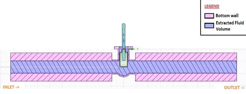
Fig: Geometry preparation

Above figure shows geometry of gate valve.

As seen in above figure, from left side i.e. inlet water with 10 Pa inlet pressure is introduced. The outlet is presented at right side. We need to calculate mass flow rate for variable lift of gate disc at outlet to compute flow factor and flow coefficient.

Meshing:

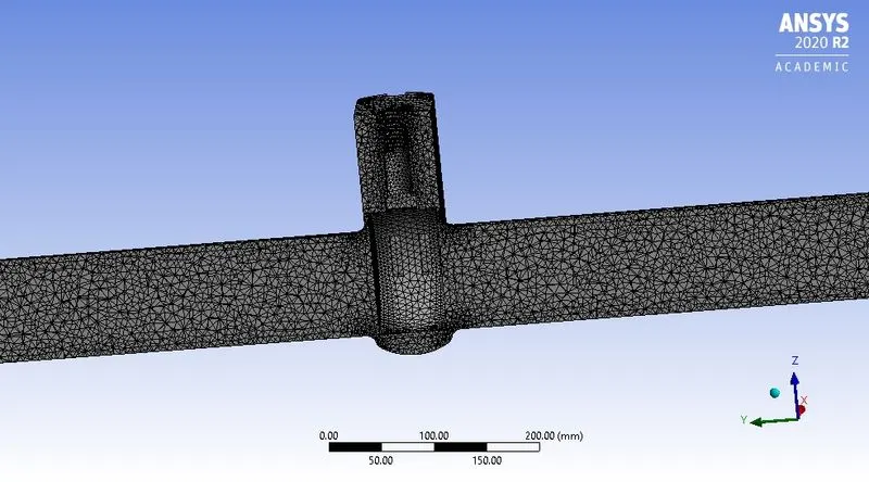
Above figure shows meshed geometry.

• Mesh element size = 7.5mm
• Maximum mesh element size = 10mm
• Number of nodes = 60101
• Number of elements = 295271

Due to computational power limitations and student license restriction, we have taken mesh element size of 7.5mm.

Further refinement in meshing definitely make result more precise and accurate.

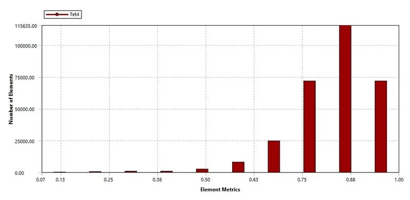Above figure shows mesh quality matrix.

As maximum number of elements are coming in between 0.5 to 1 element matrix range, hence the overall quality of mesh is considered as good meshing to perform further simulation.

Material:

The material used as a fluid is water (`H_2O`) in liquid state.

Material properties are as follows-

Density = 998.2 `(kg)/m^3`

Dynamic viscosity = 0.001003 `(Kg)/(m.s)`

Boundary condition and solving:

Pressure inlet = 10 Pa

Outlet pressure = Gauge pressure 0 Pa

From above inlet pressure we get inlet velocity = 0.1415488 m/s

As Reynolds number is greater than 2000, thus fluid flow is turbulent.

Hence consider Turbulent model for calculations.

Setting steps:-

• Enable pressure based solver
• Consider steady state simulation
• Enable gravity in '-ve' Z direction
• Put value 9.81 in gravity field
• Select `k-epsilon` turbulent model
• Enable Realizable option
• Select scalable wall option
• Choose COUPLED scheme
• And make standard initialization
• Take reference value from inlet

Post processing:

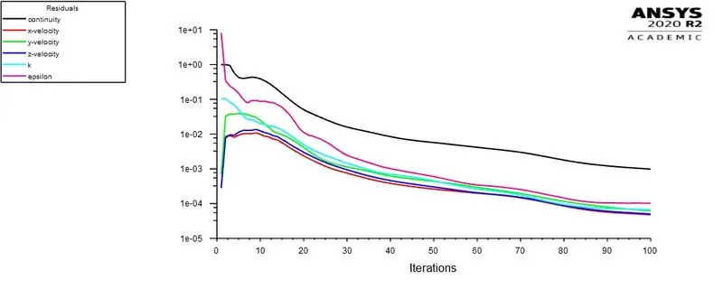
~Case 1 (10 mm lift):

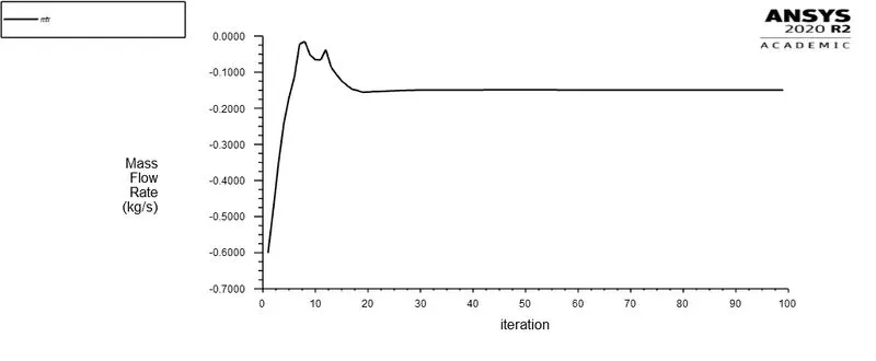Fig: Residual v/s Iteration plot	Fig: Mass flow rate at outlet

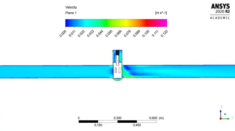
Fig: Velocity contour

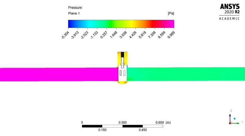
Fig: Pressure contour

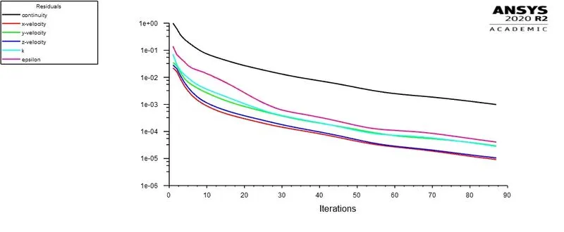
~Case 2 (20 mm lift):

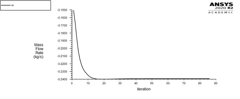Fig: Residual v/s Iteration plot	Fig: Mass flow rate at outlet

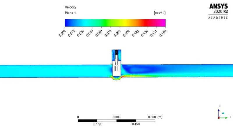
Fig: Velocity contour

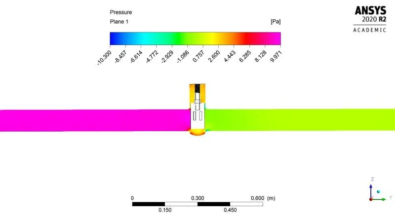
Fig: Pressure contour

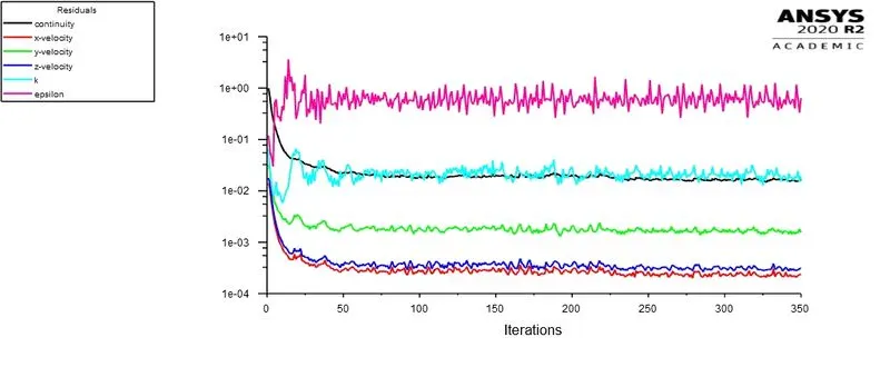
~Case 3 (30 mm lift):

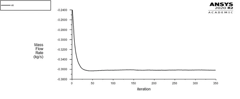Fig: Residual v/s Iteration plot	Fig: Mass flow rate at outlet

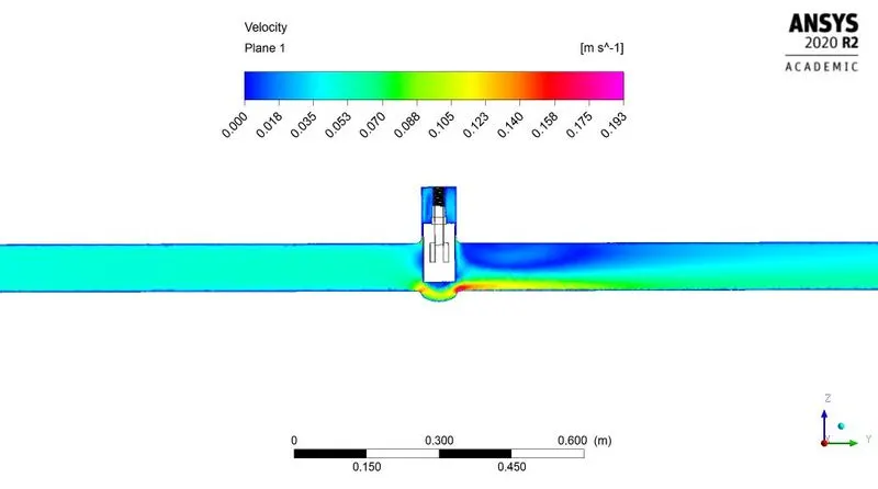
Fig: Velocity contour

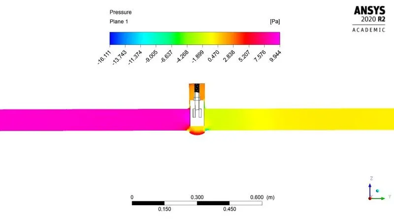
Fig: Pressure contour

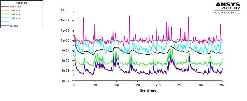
~Case 4 (40 mm lift):

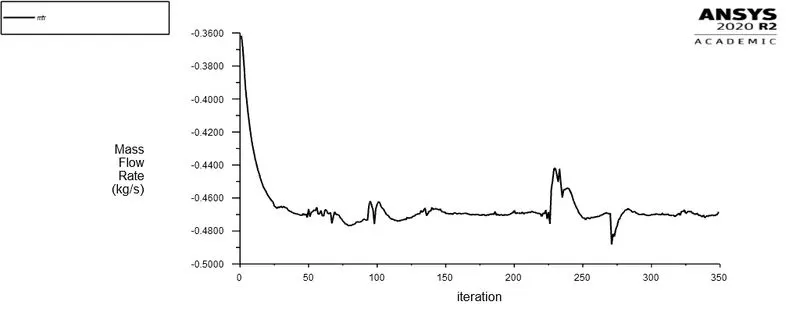Fig: Residual v/s Iteration plot	Fig: Mass flow rate at outlet

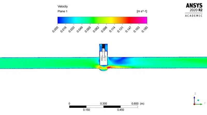
Fig: Velocity contour

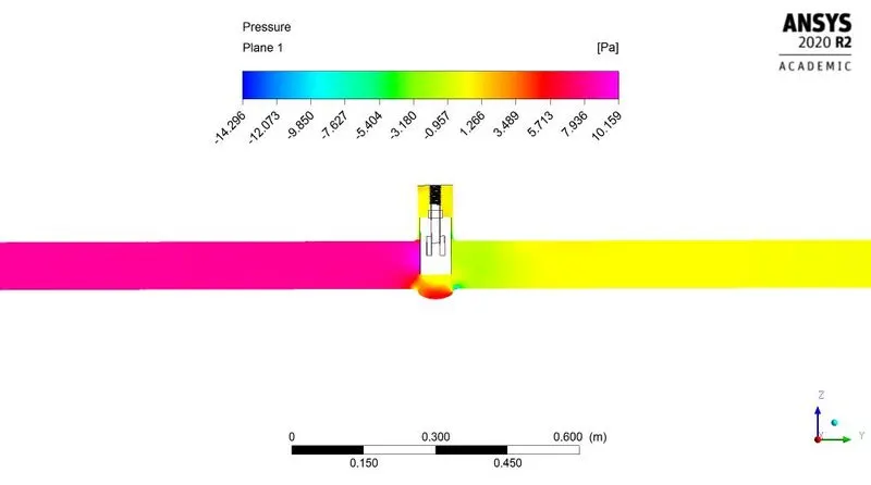
Fig: Pressure contour

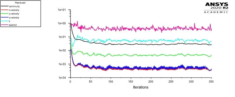
~Case 5 (50 mm lift):

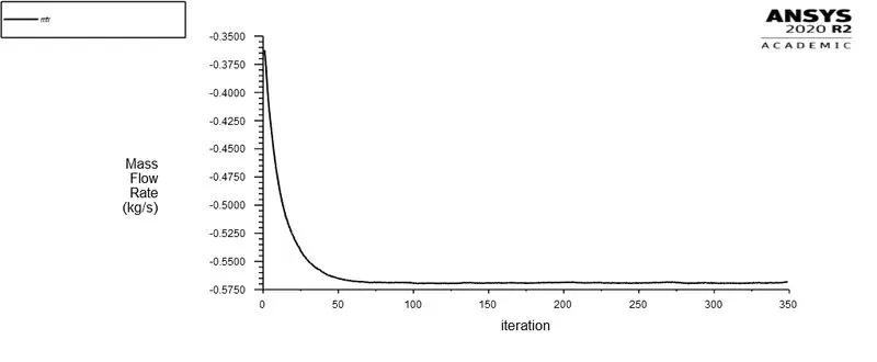Fig: Residual v/s Iteration plot	Fig: Mass flow rate at outlet

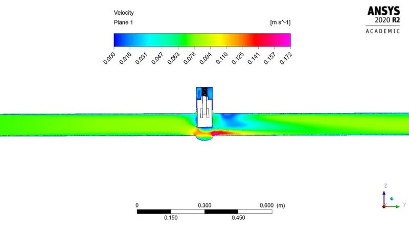
Fig: Velocity contour

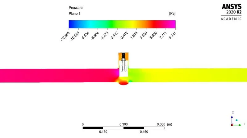
Fig: Pressure contour

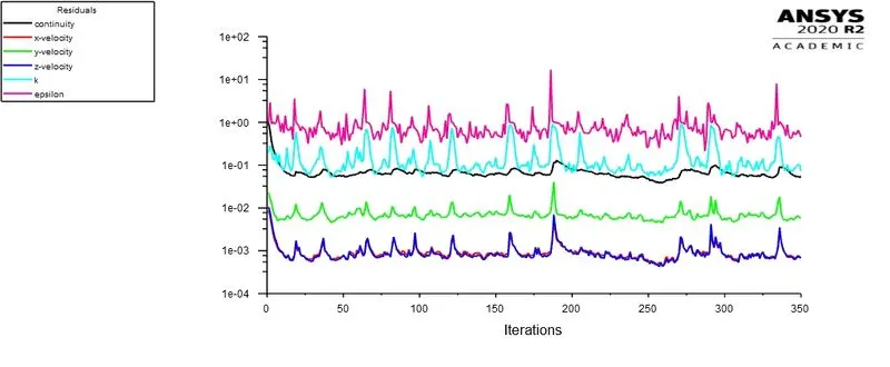
~Case 6 (60 mm lift):

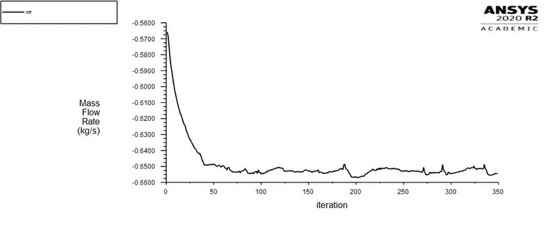Fig: Residual v/s Iteration plot	Fig: Mass flow rate at outlet

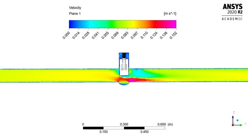
Fig: Velocity contour

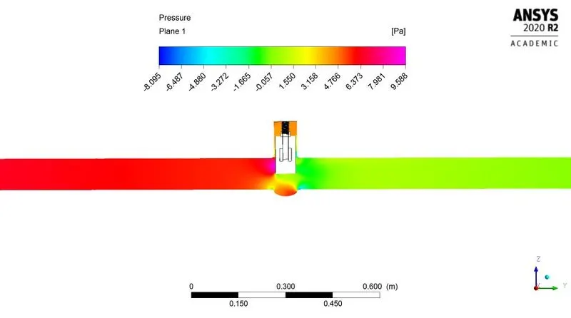
Fig: Pressure contour

~Case 7 (70 mm lift):

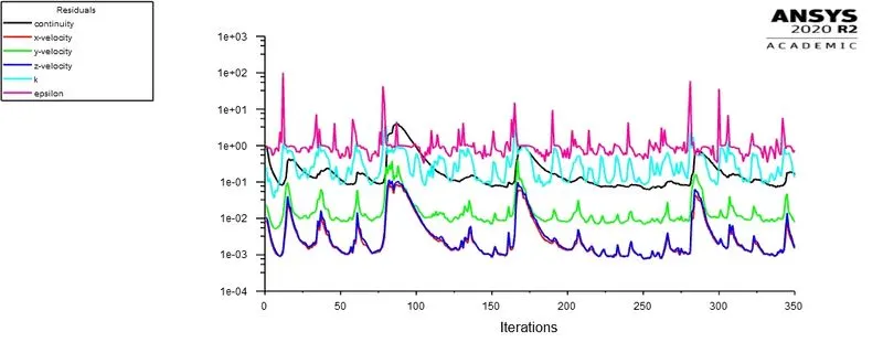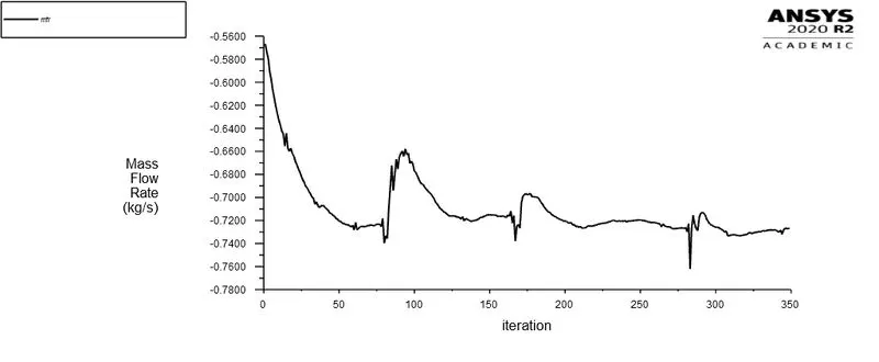Fig: Residual v/s Iteration plot	Fig: Mass flow rate at outlet

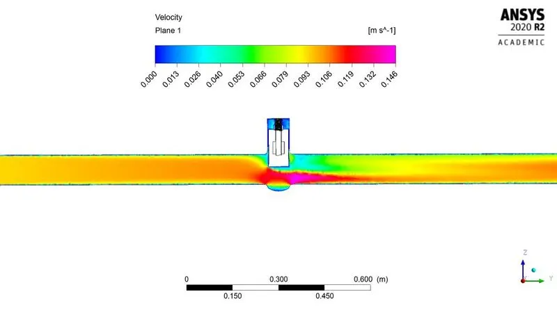
Fig: Velocity contour

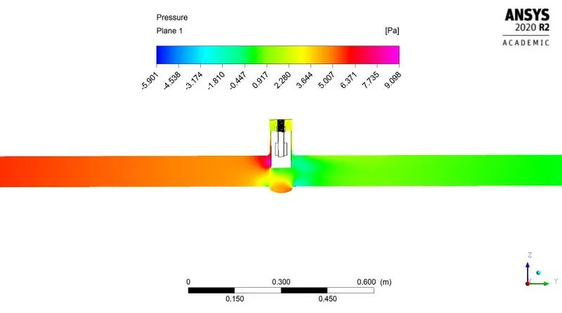
Fig: Pressure contour

~Case 8 (80 mm lift):

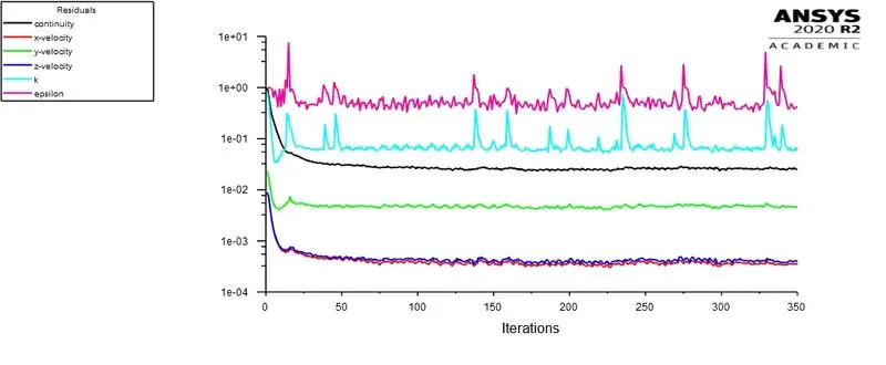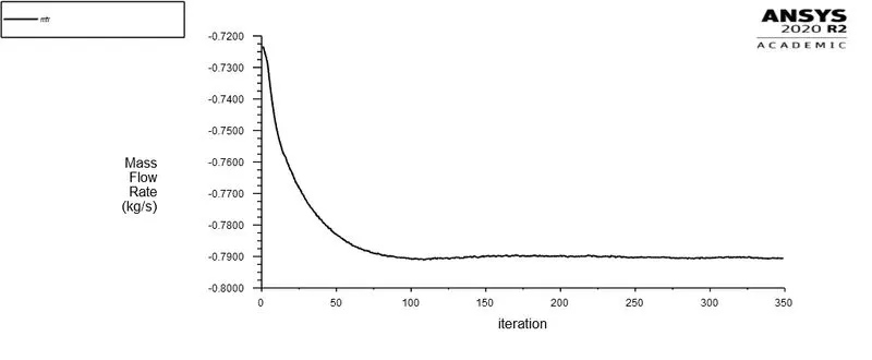Fig: Residual v/s Iteration plot	Fig: Mass flow rate at outlet

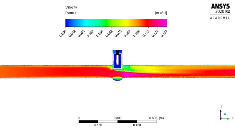
Fig: Velocity contour

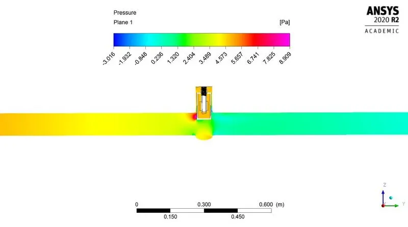
Fig: Pressure contour

As seen in above 8th case its seen that the fluid enters inside gate disc. It happens due to threads on spindle. At lift of 80mm the gap is formed between spindle and gate disc. The fluid enters inside gate disc from gap present between spindle threads and gate surface.

Calculations:

As our Reynolds number is in between `10^5` and `4xx10^7`

Hence the coefficient of friction for pipe surface can be calculated as-

`f_D=(0.0791)/(Re)^(1/4)`

`:.f_D=(0.0791)/(14087)^(1/4)`

`:.f_D=0.007261`

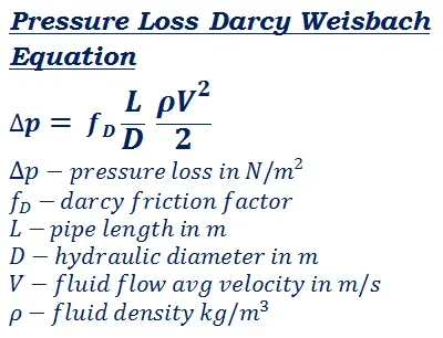
`L="Pipe length"=1.837m`

`Deltap=(0.007261xx1.837xx998.2xxV^2)/(2xx0.1)`

`:.Deltap=66.5685xxV^2`

As we know, Average velocity = 0.5*maximum velocity

Hence from above velocity contours we get maximum velocity

Hence pressure drop can be calculate as-

`Deltap=16.6421xxV_max^2`

Flow coefficient:

`Cv=Qxxsqrt((S_G)/(Deltap))`

Flow factor:

`Kv=0.865xxCv`

MATLAB code:

clear all
close all
clc

Q = [0.14918184, 0.23925383, 0.3618066, 0.47325322, 0.5676334, 0.65441511, 0.72630894, 0.790396118];
V_max = [0.122, 0.166, 0.193, 0.180, 0.172, 0.152, 0.146, 0.137];
S_G = 1;

Delta_p = 16.6421*V_max.^2;

## 1Pa = (1/6895)PSI
## 1kg/s = 21.44GPM

Cv = (Q*21.44).*((S_G)./(Delta_p./6895)).^0.5;
Kv = (0.865.*Cv);

figure 1;
plot(Cv,'-*-','color','r');
hold on;
plot(Kv,'-*-','color','b');
title("Flow coef. & Flow factor values");
legend("Flow coefficient","Flow factor");
ylabel("Magnitude");
xlabel("Sr. Number");

The above MATLAB code is provided for calculating values of pressure drop, flow coefficient and flow factor. For simplicity in calculation the above small program is created.

Result:

Sr. No.	Lift (mm)	Max velocity (m/s)	Mass flow rate @ outlet (Kg/s)	`Delta p="Pressure drop"` `(N/m^2)`	Flow coefficient `Cv`	Flow factor `Kv`
1	10	0.122	0.14918184	0.2477	533.63	461.59
2	20	0.166	0.23925383	0.45859	628.98	544.07
3	30	0.193	0.3618066	0.6199	818.1	707.66
4	40	0.180	0.47325322	0.5392	1147.4	992.49
5	50	0.172	0.5676334	0.49234	1440.2	1245.8
6	60	0.152	0.65441511	0.3845	1878.9	1625.2
7	70	0.146	0.72630894	0.35474	2171	1877.9
8	80	0.137	0.790396118	0.31236	2517.7	2177.9

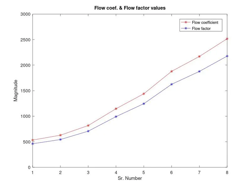
Fig: Flow coefficient & flow factor at various lift

The above plot is obtained in MATLAB after running calculation code provided above. As seen in above figure for the increasing value of lift we are getting flow coefficient and flow factor values in ascending order.

Conclusion:- From observing above all results, tables, plots and postprocessed data we can conclude that-

1. As gate disc lift increases, mass flow rate at outlet also increases.
2. As gate disc lift increases, flow coefficient & flow factor also increases.
3. In ANSYS negative mass flow rate denotes the mass is flowing out of the body.
4. Flow coefficient is one of the standards for expressing the flow capacity of hydraulic devices
5. ANSYS assist to perform parametric study which optimize time and hecticness for performing lots of iterations and study
6. Due to high velocity and lowering in pressure drop results cavitation