Literature review of RANS model

Literature review of RANS Model

Reynolds Number:- It is the non-dimensional number, as it is ratio of two similar quantities (force). The Reynolds number is expressed as ratio of inertial force to viscous force within a fluid. The Reynolds number is term, which tells behavior of fluid. As inertial force is less, the viscus force dominate flow, which gives laminar flow. If scenario gets reverse, inertial force is much higher than viscus force, the outcome we get is turbulent flow.

Reynolds number mathematically expressed as,

`Re = ("Inertial force")/("Viscous force")= (ρVL)/μ`

When we consider an engineering flow problem, most of the times it is observed that the flow is turbulent in nature. The behavior of fluid (i.e., is fluid laminar or turbulent?) is depend on Reynolds number. If the Reynolds number greater than 4000 the flow is considered to be turbulent flow and if flow is less than 2300 the flow is laminar. The flow between Reynolds number 2300 and 4000, the flow is transition flow.

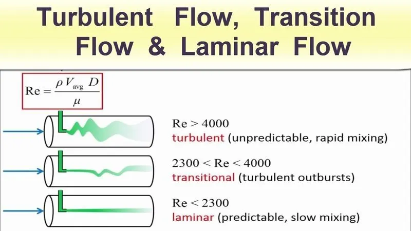Laminar flow:- Laminar flow occurs when the fluid flows in infinitesimal parallel layers with no disruption between them. In laminar flows, fluid layers slide in parallel, with no eddies, swirls or currents normal to the flow itself. This type of flow is also referred to as streamline flow because it is characterized by non-crossing streamlines. The laminar regime is ruled by momentum diffusion, while the momentum convection is less important.

Transition flow:- The transition regime separates the laminar and the turbulent flows. Transitional flow is a mixture of laminar and turbulent flow, with turbulence in the center of the pipe, and laminar flow near the edges.

Turbulent flow:- Turbulent flow is a type of fluid (gas or liquid) flow in which the fluid undergoes irregular fluctuations, or mixing. In turbulent flow the speed of the fluid at a point is continuously undergoing changes in both magnitude and direction. Turbulence is caused by excessive kinetic energy in parts of a fluid flow, which overcomes the damping effect of the fluid's viscosity. For this reason, turbulence is commonly realized in low viscosity fluids. In turbulent flow, unsteady vortices called eddies appear of many sizes which interact with each other.

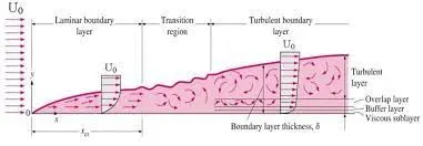The above figure shows boundary layer development in various flow regions, starting from laminar region then transition region and up to turbulent region. In a flow bounded by a wall, different scales and physical processes are dominant in the inner portion near the wall, and the outer portion approaching the free stream. These layers are typically known as the inner and outer layers. Considering the flow over a smooth flat plate the boundary layer can be distinguished into two types namely laminar boundary layer and turbulent boundary layer.

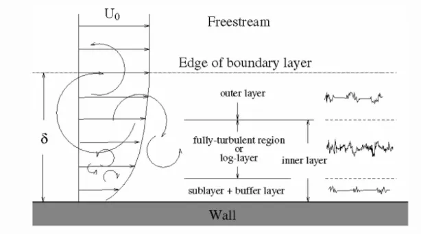
The boundary layer thickness, `delta` is the distance from the wall at which viscous effects become negligible and represents the edge of the boundary layer. At height of `delta` the flow velocity is considered to be freestream velocity `U_0`. Near to the wall the flow is influenced by the viscous effects and independent of free stream parameters, thus velocity near to wall is considered as 0.

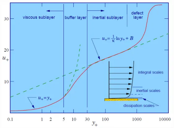Fig: Velocity profile in turbulent flow	Fig: Plot of y+ v/s u+

Turbulent flows are significantly affected by the presence of walls, where the viscosity-affected regions have large gradients in the solution variables. An accurate representation of the near wall region determines a successful prediction of wall bounded turbulent flows. So using wall function makes things easier. Using wall function, one can model the near wall region. Wall functions are nothing but mathematical equations derived empirically and used to satisfy the physics in the near wall region. The first cell center needs to be placed in the viscous region to ensure the accuracy of the results. And the first cell thickness is calculated using Y+. Where Y+ is distance from the wall measured in terms of viscous lengths and can be called as dimensionless wall distance as it is non dimensional term.

Mathematically y+ can be expressed as-

`y^+ = (y_1xxu_t)/nu`

Where, y1 = first layer thickness

`u_t=` Frictional velocity

Another non dimensional term is u+ which is called as dimensionless velocity. It can be mathematically expressed as-

`u^+ = u/u_t`

A turbulent boundary layer consists of distinct regions. From both of the above images it is seen that regions near wall and how velocity behaves in particular region near wall. It can be classified as per follows-

1. Viscous sub layer:- In the viscous layer, the fluid is dominated by the viscous effect, so it can be assumed that the Reynolds shear stress is negligible. The above layer is under y+ value of 5. The relation between non dimensional velocity and non dimensional distance can be given as-

`u^+ = y^+`

2. Buffer layer:- The buffer layer is the transition region between the viscosity-dominated region and turbulence-dominated part of the flow i.e., log law region. Viscous and turbulent stresses are of similar magnitude and since it is complex, the velocity profile is not well defined and the original wall functions avoid the first cell center located in this region. The y+ value for this region is between 5 to 30.

3. Log law layer:- In the logarithmic layer, turbulence stress dominates the flow and velocity profile varies very slowly with a logarithmic function along the distance y. For this region the y+ value needs to be greater than 30. The relationship between y+ and u+ can be expressed as-

`u ^+ = 1/κ l n ( y^ + ) + B`

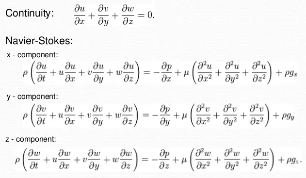
Governing equations for laminar flow:-

Turbulence modeling:-

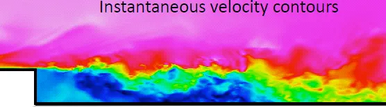
As we know in turbulence flow, the flow is always varying (Fluctuating) with respect to time. So it gets very hectic to solve Navier Stokes equations. So, instead of considering solution at instant we prefer to used time average solution.

Characteristics of turbulent flow are as follows:

1. Irregular and random
2. 3D
3. High Vorticity
4. Large Reynolds number

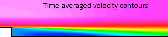The above figure shows how solution contour looks for time averaged solution and instantaneous solution. So to obtain time average solution we need to integrate governing equations over a time. So to take time averaged solution we need to apply Reynolds decomposition.

Reynolds decomposition:- If we draw plot of instantaneous velocities at various time we can obtain following figure.

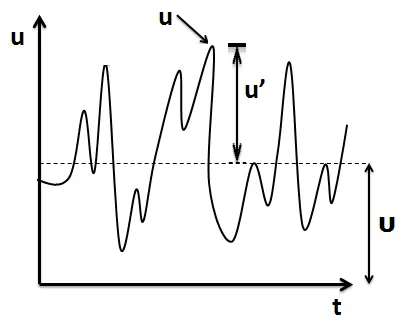It is seen from above plot that in turbulent flow the velocity is always varying with respect to time and the variation is not in any order. So by applying Reynolds decomposition we can able to calculate correct results.

Velocity at any instant can be calculated as,

`u(t)=U+u'(t)`

Where, u = Instantaneous velocity

U = Mean velocity

u' = Fluctuation in velocity

So in same fashion we can decompose functions into two parts i.e., mean quantity and fluctuating quantity. The mean quantity will always remain same at any time instant but fluctuating quantity may varies with time. Thus, using Reynolds decomposition the functions of fluid properties (parameters) can be expressed as-

`u(x,y,z,t)=baru(x,y.z)+u'(x,y,z,t)`

`v(x,y,z,t)=barv(x,y.z)+v'(x,y,z,t)`

`w(x,y,z,t)=barw(x,y.z)+w'(x,y,z,t)`

`P(x,y,z,t)=barP(x,y.z)+P'(x,y,z,t)`

As we know time integration of fluctuating term is zero.

`bar(u')=1/Tint_0^Tu'dt=0`

So now if we apply this Reynolds decomposition scheme to Navier stokes equation, we obtain RANs model i.e., Reynolds Average Navier Stokes model.

Consider 2D Navier stokes equations dor avoiding complexity.

~Now for continuity equation,

`(delu)/(delx)+(delv)/(dely)= 0`

By taking Reynolds decomposition we get,

`:.(del)/(delx)(baru+u')+(del)/(dely)(barv+v')=0`

Performing time averaging,

`:.1/Tint_0^T[(del)/(delx)(baru+u')+(del)/(dely)(barv+v')]dt=0`

`:.[1/Tint_0^T(delbaru)/(delx)dt]+[1/Tint_0^T(delu')/(delx)dt]+[1/Tint_0^T(delbarv)/(dely)dt]+[1/Tint_0^T(delv')/(dely)dt]=0`

As time average of fluctuating term is 0,

`:.[1/Tint_0^T(delbaru)/(delx)dt]+cancel[1/Tint_0^T(delu')/(delx)dt]+[1/Tint_0^T(delbarv)/(dely)dt]+cancel[1/Tint_0^T(delv')/(dely)dt]=0`

`:.[1/T (delbaru)/(delx)int_0^Tdt]+[1/T(delbarv)/(dely)int_0^Tdt]=0`

`:.(delbaru)/(delx)+(delbarv)/(dely)=0`

~Now consider momentum equation,

For x direction,

`(delu)/(delt)+u(delu)/(delx)+v(delu)/(dely) = -1/rho(delP)/(delx)+nu(del^2u)/(dely^2)`

`(delu)/(delt)+u(delu)/(delx)+v(delu)/(dely) + uxx0 = -1/rho(delP)/(delx)+nu(del^2u)/(dely^2)`

As we know, `(delu)/(delx)+(delv)/(dely)=0` So adding this term in left hand side,

`:.(delu)/(delt)+u(delu)/(delx)+v(delu)/(dely) +[u((delu)/(delx)+(delv)/(dely))] = -1/rho(delP)/(delx)+nu(del^2u)/(dely^2)`

`:.(delu)/(delt)+2u(delu)/(delx)+v(delu)/(dely) +u(delv)/(dely) = -1/rho(delP)/(delx)+nu(del^2u)/(dely^2)`

But as per product rule of derivative, `(del(uv))/(dely)=u(delv)/(dely)+v(delu)/(dely)`

`:.(delu)/(delt)+2u(delu)/(delx)+[v(delu)/(dely) +u(delv)/(dely)] = -1/rho(delP)/(delx)+nu(del^2u)/(dely^2)`

The equation can be rewritten as,

`:.(delu)/(delt)+2u(delu)/(delx)+[(del(uv))/(dely)] = -1/rho(delP)/(delx)+nu(del^2u)/(dely^2)`

Again we know, `(del(u^2))/(delx)=2u(delu)/(delx)`

`:.(delu)/(delt)+(del(u^2))/(delx)+(del(uv))/(dely) = -1/rho(delP)/(delx)+nu(del^2u)/(dely^2)`

Let us apply Reynolds decomposition and time averaging for above equation,

Hence we get,

`1/T int_0^T[(del)/(delt)(baru+u')+(del)/(delx)(baru+u')^2+(del)/(dely)[(baru+u')(barv+v')]] dt= 1/T int_0^T[-1/rho(del)/(delx)(barP+P')+nu(del^2)/(dely^2)(baru+u')]dt`

Let us expand LHS first,

`:.[1/T int_0^T(delbaru)/(delt)dt]+[1/T int_0^T(delu')/(delt)dt]+[1/T int_0^T(del(baru)^2)/(delx)dt]+[1/T int_0^T(del(u')^2)/(delx)dt]+[1/T int_0^T(delbaruv')/(dely)dt]+[1/T int_0^T(delu'v')/(dely)dt]+[1/T int_0^T(delbarvu')/(dely)dt]+[1/T int_0^T(delbarvbaru)/(dely)dt]`

`= 1/T int_0^T[-1/rho(del)/(delx)(barP+P')+nu(del^2)/(dely^2)(baru+u')]dt`

Fluctuating terms became zero,

`:.[1/T int_0^T(delbaru)/(delt)dt]+cancel[1/T int_0^T(delu')/(delt)dt]+[1/T int_0^T(del(baru)^2)/(delx)dt]+[1/T int_0^T(del(u')^2)/(delx)dt]+cancel[1/T int_0^T(delbaruv')/(dely)dt]+[1/T int_0^T(delu'v')/(dely)dt]+cancel[1/T int_0^T(delbarvu')/(dely)dt]+[1/T int_0^T(delbarvbaru)/(dely)dt]`

`= 1/T int_0^T[-1/rho(del)/(delx)(barP+P')+nu(del^2)/(dely^2)(baru+u')]dt`

So LHS becomes,

`:.[1/T int_0^T(delbaru)/(delt)dt]+[1/T int_0^T(del(baru)^2)/(delx)dt]+[1/T int_0^T(del(u')^2)/(delx)dt]+[1/T int_0^T(delu'v')/(dely)dt]+[1/T int_0^T(delbarvbaru)/(dely)dt]`

`= 1/T int_0^T[-1/rho(del)/(delx)(barP+P')+nu(del^2)/(dely^2)(baru+u')]dt`

Now solving RHS,

`:.[1/T int_0^T(delbaru)/(delt)dt]+[1/T int_0^T(del(baru)^2)/(delx)dt]+[1/T int_0^T(del(u')^2)/(delx)dt]+[1/T int_0^T(delu'v')/(dely)dt]+[1/T int_0^T(delbarvbaru)/(dely)dt]`

`= [1/T int_0^T(-1/rho)(delbarP)/(delx)dt]+[1/T int_0^T(-1/rho)(delP')/(delx)dt]+[1/T int_0^Tnu(del^2baru)/(dely^2)dt]+[1/T int_0^Tnu(del^2u')/(dely^2)dt]`

Now cancelling fluctuating terms on RHS

`:.[1/T int_0^T(delbaru)/(delt)dt]+[1/T int_0^T(del(baru)^2)/(delx)dt]+[1/T int_0^T(del(u')^2)/(delx)dt]+[1/T int_0^T(delu'v')/(dely)dt]+[1/T int_0^T(delbarvbaru)/(dely)dt]`

`= [1/T int_0^T(-1/rho)(delbarP)/(delx)dt]+cancel[1/T int_0^T(-1/rho)(delP')/(delx)dt]+[1/T int_0^Tnu(del^2baru)/(dely^2)dt]+cancel[1/T int_0^Tnu(del^2u')/(dely^2)dt]`

Re writing above equation,

`:.[1/T int_0^T(delbaru)/(delt)dt]+[1/T int_0^T(del(baru)^2)/(delx)dt]+[1/T int_0^T(del(u')^2)/(delx)dt]+[1/T int_0^T(delu'v')/(dely)dt]+[1/T int_0^T(delbarvbaru)/(dely)dt]`

`= [1/T int_0^T(-1/rho)(delbarP)/(delx)dt]+[1/T int_0^Tnu(del^2baru)/(dely^2)dt]`

After solving above equation,

`:.(delbaru)/(delt)+(del(baru)^2)/(delx)+(delbarvbaru)/(dely)= (-1/rho)(delbarP)/(delx)+nu(del^2baru)/(dely^2)-[1/T int_0^T(del(u')^2)/(delx)dt]-[1/T int_0^T(delu'v')/(dely)dt]`

When we consider u' fluctuation between 1 and -1 values, so on performing time average the fluctuating term cancel out each other and gets zero. On the other hand if we consider square of fluctuating term, it didn't cancel out and give finite value.

`:.[1/T int_0^T(del(u')^2)/(delx)dt] !=0`

But by making assumption that the flow is in boundary layer, we can neglect above term. Because in boundary layer the velocity gradient along y direction is much greater than gradient of velocity in x direction.

So above equation is,

`:.(delbaru)/(delt)+(del(baru)^2)/(delx)+(delbarvbaru)/(dely)= (-1/rho)(delbarP)/(delx)+nu(del^2baru)/(dely^2)-cancel[1/T int_0^T(del(u')^2)/(delx)dt]-[1/T int_0^T(delu'v')/(dely)dt]`

`:.(delbaru)/(delt)+(del(baru)^2)/(delx)+(delbarvbaru)/(dely)= -1/rho(delbarP)/(delx)+nu(del^2baru)/(dely^2)-[1/T int_0^T(delu'v')/(dely)dt]`

`:.(delbaru)/(delt)+(del(baru)^2)/(delx)+(delbarvbaru)/(dely)= -1/rho(delbarP)/(delx)+1/(rho)(del)/(delu)[mu(delbaru)/(dely)-(rho)/T int_0^T(u'v')dt]`

The final equation is expressed in more suitable way as follows-

`ubrace[(delbaru)/(delt)+(del(baru)^2)/(delx)+(delbarvbaru)/(dely)]_("Rate of momentum change")= ubrace[-1/rho(delbarP)/(delx)]_("Isotropic stress due to pressure field")+1/(rho)(del)/(delu)[ubrace(mu(delbaru)/(dely))_"Viscous stress"-ubrace[(rho)/T int_0^T(u'v')dt]_"Reynolds stress"]`

The velocity fluctuations are found to give rise to additional stresses on the fluid, the so-called Reynolds stresses. Reynolds stresses arise from the averaging procedure used in deriving the RANS equations. They are the additional unknowns that create the closure problem (not enough equations to solve unknowns).

The Reynolds stress can be given as-

`tau_(ij)^(Re)=-rho(bar(u_i'u_j'))`

Reynolds stress tensor can be giveen as-

`tau_"ij"=[[tau_"xx", tau_"xy", tau_"xz"],[tau_"yx", tau_"yy", tau_"yz"],[tau_"zx", tau_"zy", tau_"zz"]]=-rho.[[bar((u')^2), bar(u'v'), bar(u'w')],[bar(v'u'), bar((v')^2), bar(v'w')],[bar(w'u'), bar(w'v'), bar((w')^2)]]`

It is seen from many results, the RANs equations are such that their solutions can never converge to time-averaged solutions to the Navier Stokes equations except in the case of availability of exact Reynolds stresses, which can be obtained only via DNS.

There are several different ways by means of which RANS models are classified. One of the more common is in terms of the number of additional PDEs one must solve beyond those of the Navier Stokes equations.

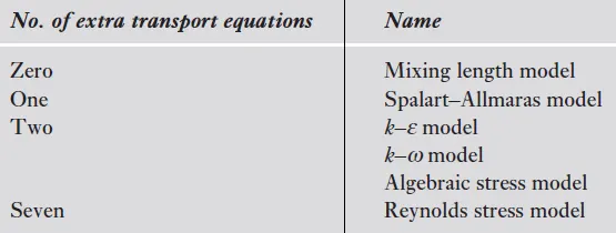
Generally, in today's practice, by using above models the turbulence flow is solved.

Turbulent viscosity or Eddy viscosity:

The turbulent transfer of momentum by eddies creates internal fluid friction. It is the fundamental idea of how we define viscosity in turbulent flow i.e., internal fluid resistance. Eddie Viscosity is an imaginary concept as it is just a number that quantifies the diffusion of a field, such as, momentum or thermal energy or a component, due to the turbulence. The Eddie Viscosity term was posed for making the things simpler. When the flow becomes turbulent, diffusion mechanism is not only performed by molecular motions, but also it is going to be highly intensified by eddies motions. Therefore, while modeling the turbulence using eddy viscosity models, we need to intensify diffusion coefficient by adding turbulent viscosity to the molecular one.

Molecular viscosity:

It is a fluid property and is same as dynamic viscosity. Dynamic viscosity is nothing but resistance to the movement of one layer of fluid over the adjacent layer (It happens due to cohesive force between fluid molecules). It is one of the most important fluid property which is easy to measure and independent of geometry. Molecular viscosity is the transfer of mass momentum motion solely by the random motion of individual molecules not moving together in coherent group.

Difference between molecular and eddy viscosity:-

1. Eddy viscosity is imaginary concept and Molecular viscosity is physically presented in fluid.
2. Turbulent viscosity is non linear while laminar viscosity is linear in nature.
3. Calculating turbulent viscosity is complex but computing molecular viscosity is simple
4. Turbulent viscosity is dominant in high Reynold number region and molecular viscosity is dominant in low Reynolds number region.
5. Turbulent viscosity is present in turbulent flow only whereas molecular viscosity is present in all kind of flow.
6. Turbulent viscosity depends upon fluid flow but molecular viscosity depends upon fluid properties.

Reference:-

1. Turbulent boundary layer
2. Derivation of Reynolds Averaged Navier Stokes Equations
3. An Introduction to CFD Finite volume method By Versteeg and Malalasekera