Geometry cleanup, boundary flagging, no hydro and full hydrodynamic simulation of S18 PFI Engine using Converge CFD

Aim:-> To perform CFD simulation of PFI engine including geometry cleanup, boundary flagging, no hydro simulation and full hydrodynamic simulation.

Theory:-

The purpose of typical internal combustion engines is to produce work by converting chemical energy to mechanical energy. In internal combustion engines chemical energy in the fuel is converted by burning or oxidizing the fuel inside the engine. After the heat from combustion causes rapid pressurization of the gaseous combustion products in the combustion chamber, causing them to expand and drive a piston rapidly, which turns a crankshaft to produce mechanical energy.

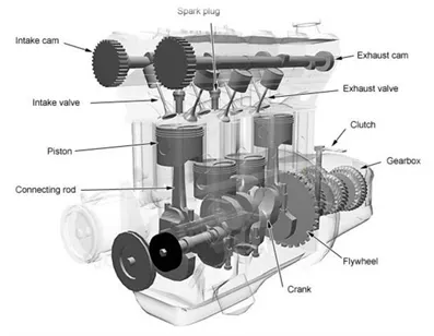There are two kinds of internal combustion engines currently in production: the spark ignition gasoline engine and the compression ignition diesel engine. Most of these are four-stroke cycle engines, meaning four piston strokes are needed to complete a cycle. The cycle includes four distinct processes: suction, compression, combustion and power stroke, and exhaust. In 1^st stroke the charge get sucked into combustion chamber, in 2^nd the charge get compressed, 3^rd stroke is power stroke where actual combustion takes place (it may happened due to excess compression in CI engine or spark ignition in case of SI engines) which gives power output and in last 4^th stroke combustible gases inside chamber are thrown out from chamber.

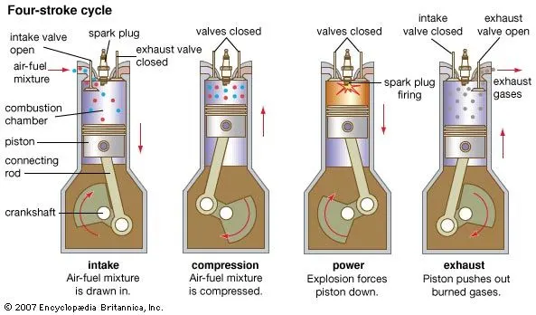Spark ignition gasoline and compression ignition diesel engines differ in how they supply and ignite the fuel. In a spark ignition engine, the fuel is mixed with air and then inducted into the cylinder during the intake process. After the piston compresses the fuel-air mixture, the spark ignites it, causing combustion. The expansion of the combustion gases pushes the piston during the power stroke. In a diesel engine, only air is inducted into the engine and then compressed. Diesel engines then spray the fuel into the hot compressed air at a suitable, measured rate, causing it to ignite.

Fuel injection:-

Fuel injection is the process of introducing fuel in an IC engine, most commonly injection process is achieved using injector. In passenger car petrol engines, fuel injection was introduced in the early 1950s, and gradually gained prevalence until it had largely replaced carburetors by the early 1990s. The primary difference between carburetion and fuel injection is that fuel injection atomizes the fuel through a small nozzle under high pressure, while a carburetor relies on suction created by intake air accelerated through a venturi tube to draw the fuel into the airstream. In an IC engine charge is created i.e., mixture of fuel and air is created for combustion. Mixture formation can be achieved in two ways for internal combustion engines. 1st one is internal mixture formation, and 2nd one is external mixture formation. A fuel injection system that uses external mixture formation is called a manifold injection system; there exist two types of manifold injection systems: multi-point fuel injection (port injection), and single-point fuel injection (throttle-body injection). Internal mixture formation systems can be separated into direct, and indirect injection systems. There exist several different varieties of both direct and indirect injection systems, the most common internal mixture formation fuel injection system is the common rail direct injection system.

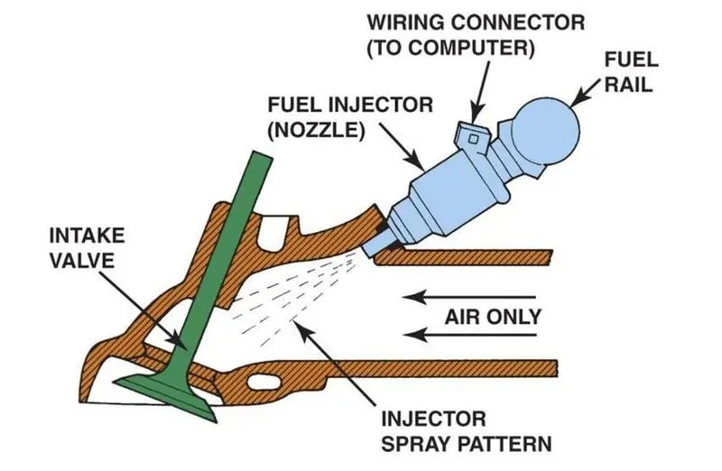As per our current case we are only focusing on port fuel injection system. In Port fuel injected internal combustion engine case the fuel is injected into the intake port (prior valve and combustion chamber) so that it gets mixed with the incoming air. The fuel injectors in PFI engines are typically mounted in the intake manifold and the charge is sucked into the cylinder as the intake valve opens.

Spray modelling:-

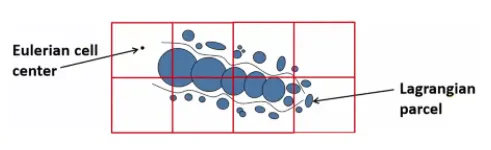
CFD modeling of spray injection and mixture formation in an IC engine is a multi-component multiphase problem which involves liquid fuel and the various species that participate in mixture formation. Generally, the gas phase is treated in an Eulerian fashion and liquid phase is treated in Lagrangian fashion. The interaction between the phases is accounted for by source terms in the Eulerian gas phase.

A well known and extensively used approach in spray modeling is the Discrete Droplet Method (DDM) which treat the spray in a Lagrangian framework. This method solves ODE’s for momentum, heat and mass transfer of a cluster of particles referred to as parcels. Each parcel is represented by a group of non-interacting droplets with identical properties. A large number of parcels combinedly defines spray behavior.

When fuel is injected through nozzle in intake manifold, it is in form of liquid spray (made of number of droplets) those droplets get interacts with the surrounding air (Air coming from inlet), a specific amount of drag force is generates on spray droplets. This action causes disturbances and due to propagation of such disturbances spray breaks up i.e., atomization happens. A liquid gets break down into small parcels which is termed as primary breakup and these small parcels again break up even further to tiny parcels is termed as secondary breakup.

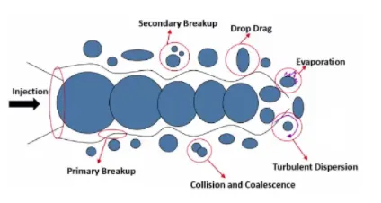When spherical parcels interact with air, their shapes get affected by flow velocity of air which results in varying speed of vaporization this effect is called as drop drag. And reduction in droplet size is described with evaporation of parcels. Experimentally it is seen that the evaporation of a droplet follows a d² law which is as given follow.

`d^2 = d_0^2 - betat`

Where, `d_0 ="Initial drop diameter"`

`d="Diameter of drop after evaporation at time t"`

`beta="Coefficient of evaporation for fuel"`

The coefficient `beta` is function of temperature, pressure and chemical concentration of fuel.

O'Rourke model:-

The model of O’Rourke considers binary collisions and collision can only occur if and only if the two parcels are situated in the same computational cell. The expected number of collisions is expressed by the following relation.

`barn = |U_(d1)-U_(d2)|pi(r_1+r_2)^2n_2/(V_"cell")Deltat`

Here larger parcel is denoted by index 2 which is also known as collector and smaller parcel denoted by index 1 is known as droplet. 'U' is relative drop velocity and 'r' is radii of drop. `n_2` is number of droplets in collector. `V_"cell"` is cell volume and `Delta t` is time step. For this model the probability of collision follows Poisson's distribution.

Sage combustion model:-

Converge provides varieties of solvers to simulate the combustion phenomenon in an IC engine. Converge provides SAGE detailed chemistry solver to simulate combustion in detailed manner. It uses local conditions to calculate reaction rates based on the principles of chemical kinetics. As we know a chemical reaction mechanism is a set of the number of elementary reactions that describe an overall chemical reaction. The combustion of different fuels can be modeled by changing the chemical mechanism. SAGE calculates the reaction rates for each elementary reaction while the CFD solver solves the transport equations. The SAGE solver is fully coupled to the flow solver, but the chemistry and flow solvers parallelize independently of one another, which speeds up the simulation. With the appropriate mechanism, the SAGE solver can predict a wide range of cases e.g., premixed, non-premixed, partially premixed, multiple fuels, emissions modeling. Though the SAGE is detailed and time consuming, Converge included some features like ‘multizone’ to reduce computational cost and time.

Simulation acceleration techniques used:-

• In order to accelerate the detailed chemistry calculations, kinetics is not solved in cells that fall below a minimum cell temperature and a minimum mole fraction. The minimum mole fraction is the total mole fraction of CO, H2, and the hydrocarbon species in fuel. The minimum mole fraction includes more than just the hydrocarbon species to allow carbon monoxide chemistry to take place in computational cells that do not include hydrocarbon species.

• Use of Jacobian matrix calculations in SAGE chemistry solver speed up simulation.

• Adaptive zoning is a technique through which user can accelerates the chemistry calculations by grouping together similar computational cells and then solves the equations using chemistry solver once per group rather than once per cell. As we know at any given time, each cell has a unique thermodynamic state. Based on the thermodynamic states of the cells, adaptive zoning technique groups the cells into a group called as zone. In a particular zone there might be multiple cells which possess similar properties like temperature and chemical composition. The thermodynamic state of each zone is based on the average temperature and composition of all of the cells in that zone.

Procedure for geometry preparation:-

• Import .stl geometry file provided by Skill Lync institute.
• Check geometry and add multiple (15 to 16) boundaries.

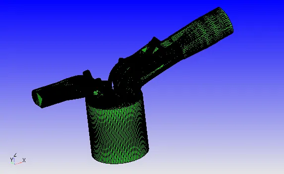
• Now click on diagnosis, to check problems in geometry.

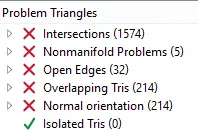
From above figure it is seen that there are many problems present in geometry. So we need to eliminate all of these problems to get started for simulation.

• Click on open edges in above diagnosis box, it will show you open edges in geometry.

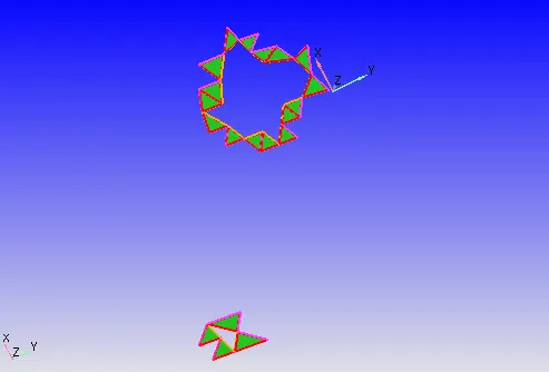
• Now select edge selector tool and choose 'by open edges' option which allows you to select open edges. Then patch the holes using patch (p) command.

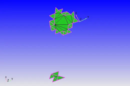
Similarly fill (patch) all the open edges.

• Select triangle selection tool with 'by angle' method. Choose any triangle in piston surface. Then add that in boundary condition with naming as piston.

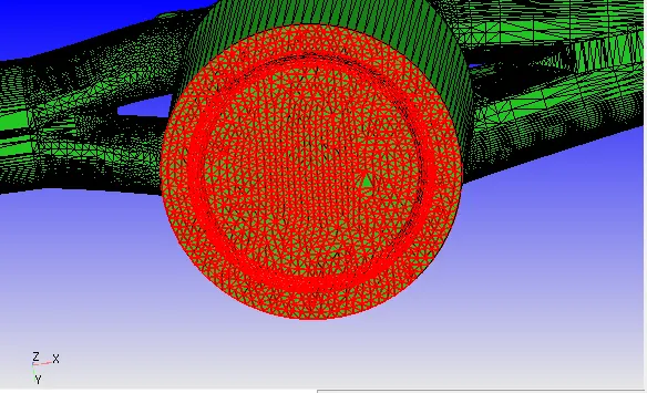
• Then try to add liner as new boundary condition. But When we try to select liner only using by angle method, its selecting liner, cylinder head with intake port. So, to select only liner let us create fence. Due to fence, we get additional option to select inside fence. It will help to create liner as single boundary condition.
• Now select liner using 'by boundary fence' method and add it in new boundary condition (BC). Give name as liner to new BC.

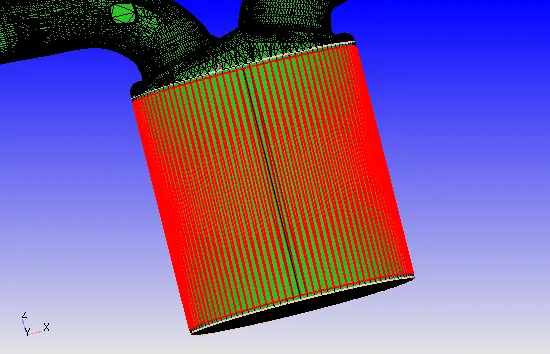
Thus, by adding this liner into new BC. Check again problems in geometry using diagnosis tool.

• Check nonmanifold problems by clicking on it. It will show problem.

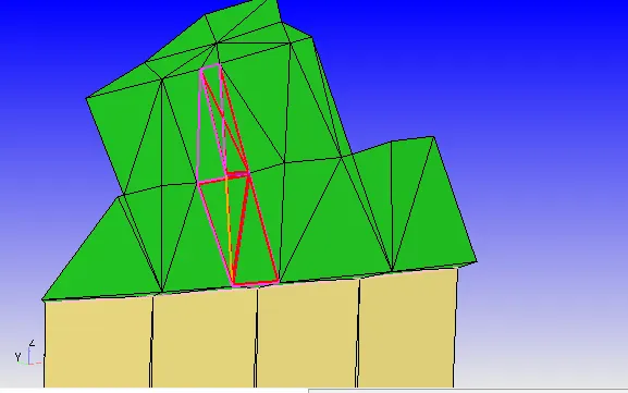
Now to eliminate above problem, delete overlapping triangles. It will create gaps with open edges. Then use simply patch tool to fill gaps between triangles. Using this method, we will get smooth geometry at that location.

• Now hit on normal orientations problem, it will show problem faces. Hit on normal toggle to see normal direction. This problem happens due to wrong direction of normal. It is necessary for all triangles that their normal should be in same direction and the pointing direction must be towards fluid. The problem can be resolved by reversing direction of triangles in correct way. To reverse direction select any triangle with wrong normal direction and by using transform option for normal change direction of normal.
• Again, diagnose the problems, it is seen only intersections problem are present now.
• Hide liner and piston to view inside parts like spark plug.
• Now check to select spark plug only. But it is not alowing to select spark plug alone. With sparkplug cylinder head and liner also getting selected. So to select sparkplug alone create fence around spark plug. And then by using method of selection by boundary fence. Now it is possible to choose spark plug alone. Add it to new BC and name it as spark plug.

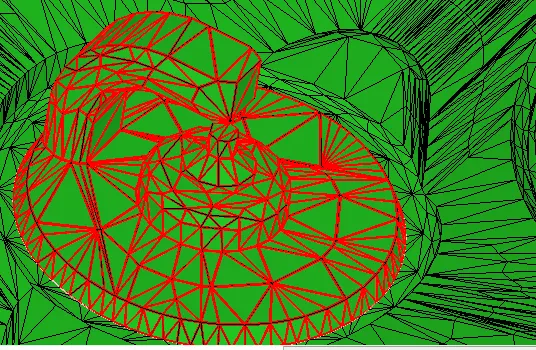
Again select only top triangles which are at end of spark plug, add them to new BC and name it as spark plug end.

• Hide triangles at end of inlet valve which are intersecting with cylinder head. Now create fence at attachment location between intake port and cylinder head.

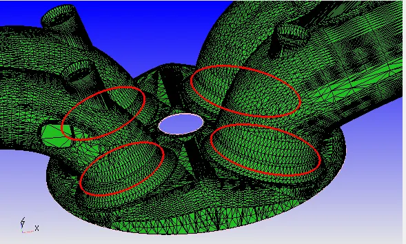
Then choose option 'by boundary fence' to select triangles of cylinder head. But before that we need to reconstruct fences from boundary.

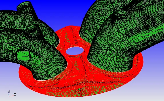
By doing above process we can able to pick cylinder head alone. Then add it to new BC and give name as cylinder head.

• Now create inflow and outflow at appropriate locations. And add them to new boundary with respective names.
• Select exhaust port triangles using triangle selection with 'by boundary fence; method. And add it to new BC give name as exhaust port.
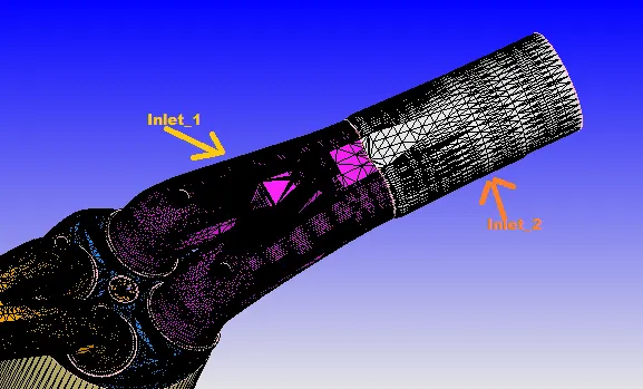
• Now divide inlet port in two sections. First one contains inflow and second part contains inlet ports. The dividing can be done by creating fence. The nearer part of cylinder can be considered as inlet port 1 and other is inlet port 2.

• Now hide exhaust port, inlet port and cylinder head, so we can take look of inlet and exhaust valves.
• Now using fence tool divide exhaust port and inlet port in three parts. 1st is top of the valve, 2nd is angled surface of valve and 3rd is bottom face of valve.

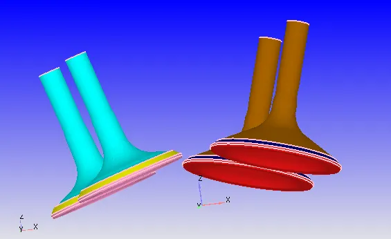
From above image it is seen that the 4 valves are colored in 6 color. Where 2 inlet ports are in same color and 2 exhaust port are in same color.

• Now once check geometry using diagnose tool, still it showing intersection errors. When we check that it is see, inlet valves are intersecting with cylinder head.
• So check the direction normal in which inlet valve is reciprocate. It can be done by direction measure tool. In that choose arc normal option. Now pic any three points on arc and enter direction vector obtained from above operation.
• Then translate inlet valve along that direction with small distance. So, it will make both surfaces distinct and after this check geometry for problems using diagnose tool. And it is seen that all errors are gets resolved. Which means we are now able to perform simulation.

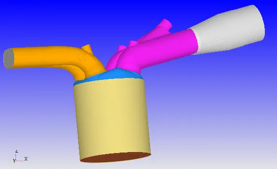
Hence, after boundary flagging, the obtained geometry is shown in above figure.

• As we have completed geometry cleanup and boundary flagging, then now let us start with the case setup.

Procedure to setup no hydro simulation:-

• Select application type as crank based IC engine.
• Enter the parameters for simulation as shown in below figure.

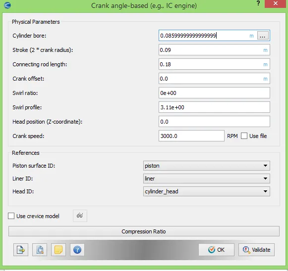
After providing physical parameters, give references with appropriate boundary conditions.

• Add therm.dat (thermodynamic data) file in gas simulation window.
• Then add reaction mechanism file in reaction mechanism window.

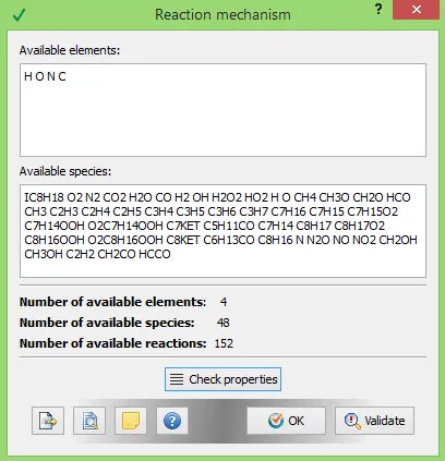
Hit on check property, if there is no error then start with next step of problem setting.

• Set the run parameters. Use no hydro simulation case as we only wanted to check mesh motion now.

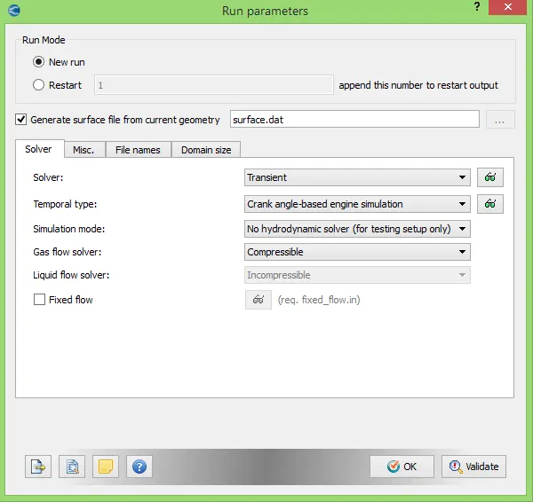
Set parameters as shown in above figure.

• Now set the simulation parameters.

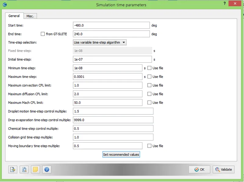
After this set solver parameters with density based solver.

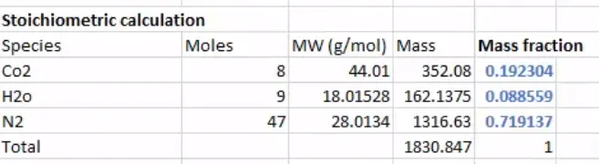
• Let us calculate mass fraction for each element in fuel.

Fuel chemical equation can be given as-

`C_8H_18+12.5(O_2+3.76N_2)<=>8CO_2+9H_2O`

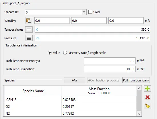
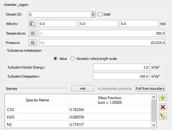
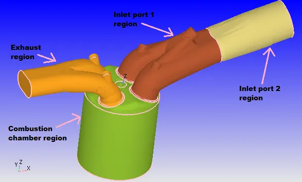
• Let us create regions now.

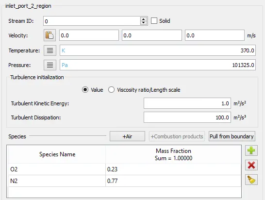Fig: Region definition for inlet_1	Fig: Region definition for inlet_2
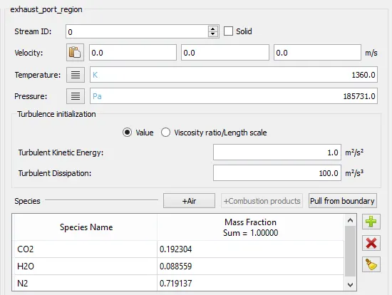Fig: Region definition for combustion cylinder	Fig: Region definition for exhaust

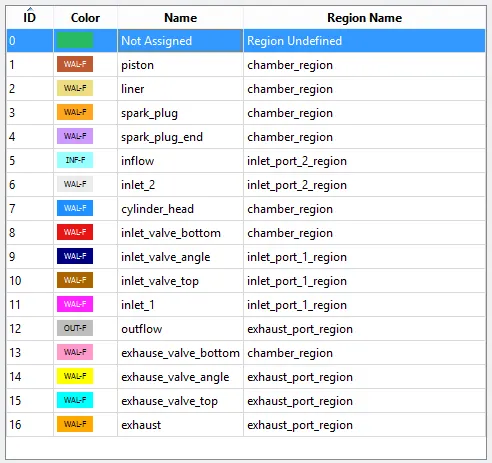
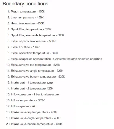
• Now provide boundary conditions-

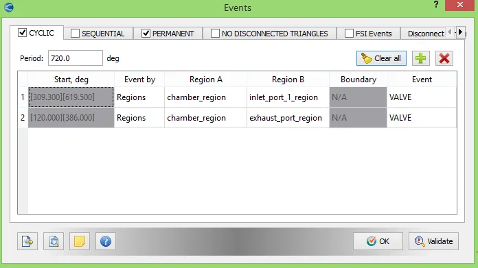
• For closing and opening the valve let us create events as follows.

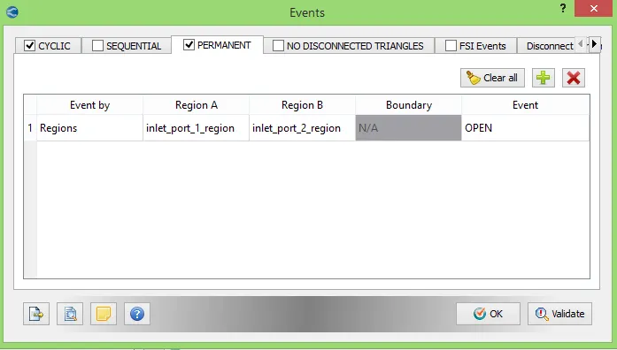The 2nd picture shows event created between inlet region 1 and inlet region 2. From inlet region 2 air is introduced and in inlet region 1 the fuel gets mixed with air to create charge.

• Then select RNG k epsilon as turbulence model.
• Set base grid with 0.004m element size in all direction.
• Set output parameters and output writing parameters.
• Export the input files and perform simulation.

While setting up problem we have provided small gap in between engine valves (inlet and exhaust valves) and cylinder head. In real world the engine valves are in contact with the cylinder head because to restrict heat transfer from engine cylinder so that the engine does not lose its thermal efficiency and also to dissipate the heat from cylinder walls to cylinder head. In real engine for valve motion spring and retainer is used but in case of simulation we didn’t included spring and retainer, so providing gap will make things simple to select face of valve and engine head.

If gap is much big the heat gets transferred through engine cylinder to intake manifold and due to high temperature in intake manifold the pre combustion may takes place in intake manifold (i.e., before inlet valve) which is not desirable.

Animation of no hydro simulation:-

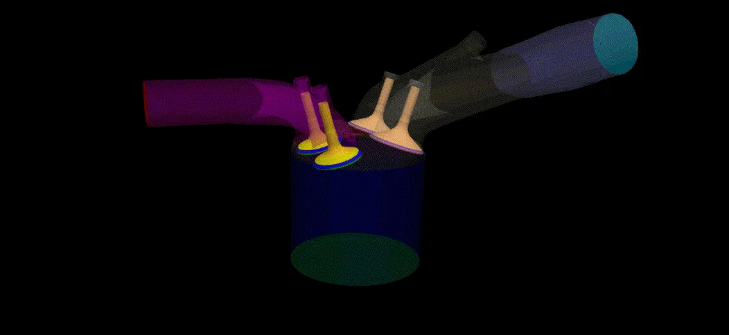
The above animation showing valve movement with respect to piston movement. It is seen that the animation is including all four strokes. On the right side of animation intake port is present and on left side exhaust port is present.

Running simulation in no hydrodynamic solver mode excludes solving models like the spray, combustion, and transport equations. Instead, this type of simulation checks surface motion and grid creation as one of the most important requirements in engine is that boundaries which means engine parts should not intersect during the simulation. And by performing no hydro simulation one can verify that your setup meets this requirement.

As seen from above no hydro simulation animation it is confirmed that problem problem and geometry seetings are accurate. Hence we can perform full hydrodynamic simulation now.

Procedure to setup full hydro simulation:-

• Enable parcel simulation from material tab.
• Now open parcel simulation tab and click on predefined liquids. Select IC8H18 i.e., iso-octane as fuel for simulation purpose. Generally, the material is selected on the basis of properties which are changing with respect to temperature.

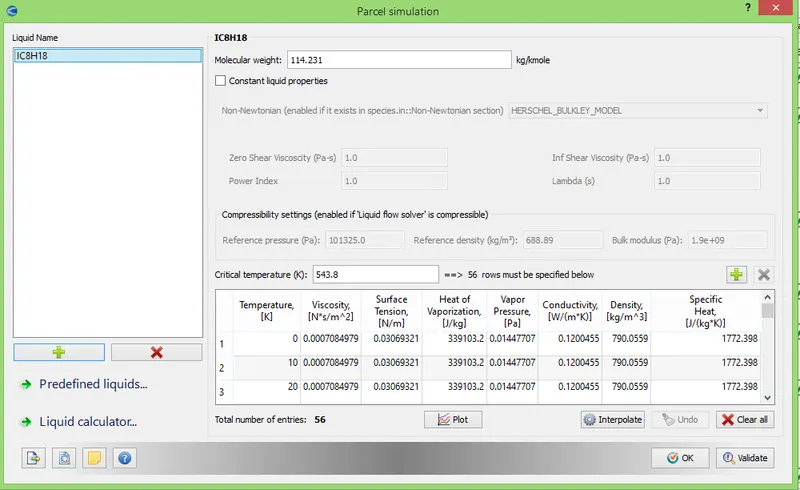
The reason behind selecting iso octane in our condition as it possess properties similar to gasoline fuel.

• Then click on species it will open species window and then select parcel tab which is inside species window. Now add parcel species from query available list which is nothing but iso octane only.
• Open run parameter window. In previous case for checking mesh generation, we have used no hydro simulation. So, for current case change it to full hydro simulation which now includes solving of Navier Stokes equation.
• Now open physical models then include combustion modelling and spray modelling by selecting check box.
• Now start with spray modelling.
• Provide general settings of spray modelling as per following figure.

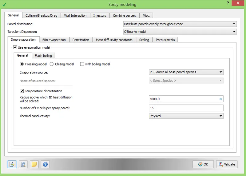
Choose parcel distribution in nozzle, for current condition it is set to 'Even parcel distribution throughout the cone'. Also Set turbulent dispersion model to 'O'Rourke model'. Under drop evaporation model, provide evaporation source as given n above figure. One can use temperature discretization for parcels which definitely increase simulation accuracy. In our case to as computation cost is major constraint so we have set very high radius value for drop.

• Now open 'Collision/Breakup/Drag' tab under spray modelling. Set Collision model as 'NTC collision' and ask for 'post collision outcomes'. Allow collision meshing at level 2 and use 'Dynamic drop drag' as drop drag model.
• Open tab of wall interaction.

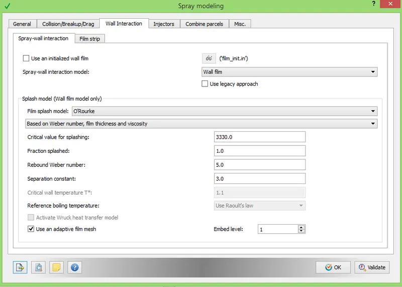
Provide values as shown in above figure.

• Then open injector tab and add injector.
• Then start editing injector properties. Add Parcel species as iso octane and provide profile for injector rate as follows.

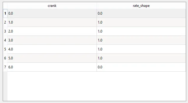
Here we are providing trapezoidal rate shape. It is cyclic and came in action at time of injection.

• Then open up model tab for injector. Check on 'Kelvin Helmholtz model' and 'Ryleigh Taylor model'. Also turn on 'Discharge coefficient model' with discharge coefficient value of 0.8. Then click on set recommendation for and select 'Gasoline PFI' which provide reference constant values for above model.

Injection Parameters:-

We have injection parameters as follows,

1. Fuel flow rate = 7.5e-4 Kg/second
2. Injection start time = -480.0
3. Injection duration = 191.2
4. Fuel temperature = 330K

• Then provide values for injection time as per above injection parameters.

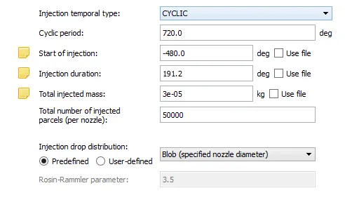
The above figure gives timing for injection. Injection start at -480 degree and ends at 191.2 degree. Total injected mass represents mass injected in kg per cycle and it can be calculated as-

As we know number of RPM for engine are 3000 which means per second 50 rotations.

So for 50 rotations the degrees covered are 18000 degrees per seconds.

So as per following injection parameters, Fuel flow rate = 7.5e-4 Kg/second

Hence for 18000 degrees 7.5e-4 kg is injected. In 1 cycle, it covers 720 degrees.

Hence, `720/18000=x/(7.5e^-4)`

`x=(720xx7.5e^-4)/18000=3e^-5`

So total injected mass per cycle is provided as 3e-5 kg.

• Provide the value of constant temperature 330 k.

Nozzle positions

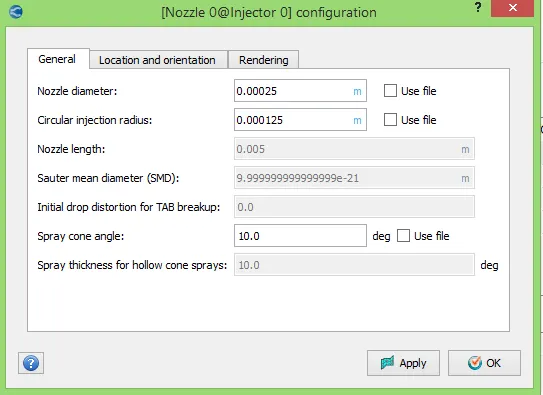
Nozzle diameter = 250 micro-meter

Circular injection radius = Nozzle radius

Spray cone angle = 10

1. Nozzle 0
   1. center 0.0823357 0.00100001 0.07019
   2. Align Vector -0.732501 0.210489 -0.647408
2. Nozzle 1
   1. center 0.0823357 -0.00099999 0.07019
   2. Align Vector -0.732501 -0.210489 -0.647408
3. Nozzle 2
   1. center 0.0823357 -0.0004 0.07019
   2. Align Vector -0.5 -0.2 -0.647408
4. Nozzle 3
   1. center 0.0823357 0.0003 0.07019
   2. Align Vector -0.5 0.2 -0.647408

• Add the 4 nozzles under nozzle tab of spray modelling window. Click on edit and add the parameters as given above.

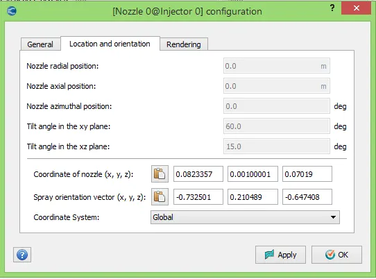Create all the four nozzles with nozzle parameters as shown in figure. After creating nozzles successfully user can view it in geometry.

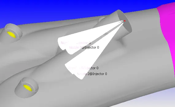
And click on validate, if any warning or error arises then solve that error.

• Under the spray modelling there are some tools. Select tool "Validate nozzle location" which will show user that nozzles are inside computational domain or not.
• Select different tool named as "Spray rate preview", so we will get-

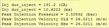
It is seen that we obtain peak pressure and velocity for injection at provided injection parameters.

• As spray modelling is completed, lets start combustion modelling.
• Add fuel species as iso octane. Provide combustion timing in degrees from -17 to 130 degrees.
• Select combustion model as SAGE combustion.

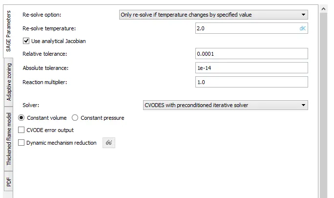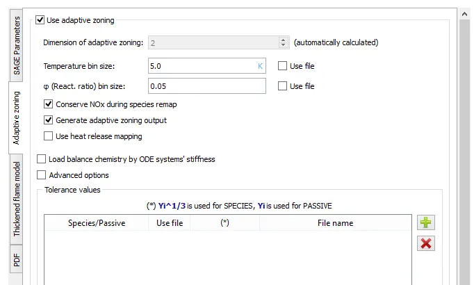
Set SAGE combustion parameters as shown in above figures and validate them.

• Now add Source/sink modelling from physical models. The reason for adding this model is to add energy source (ignition source) in engine simulation.

Spark Ignition Parameters

1. Start of spark = -15 deg
2. Spark duration = 10 deg
3. Spark location = -0.003 0 0.00915
4. Spark radius = 0.0005m

With above parameters, add source of 0.02 J in sphere shape for -15 to -14.75 degrees. Similarly add another source with same values for -15 to -5 degree.

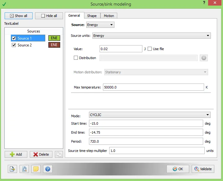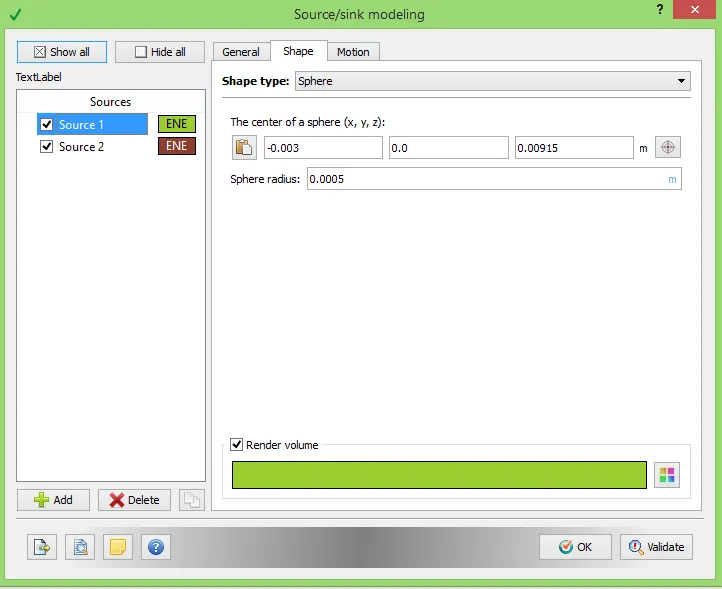It is seen from studies that when spark gets generate through spark plug, initially energy is much higher and then it reduces a bit and then becomes stable that's why we have provided two energy sources. After setting up spark let us check it in geometry.

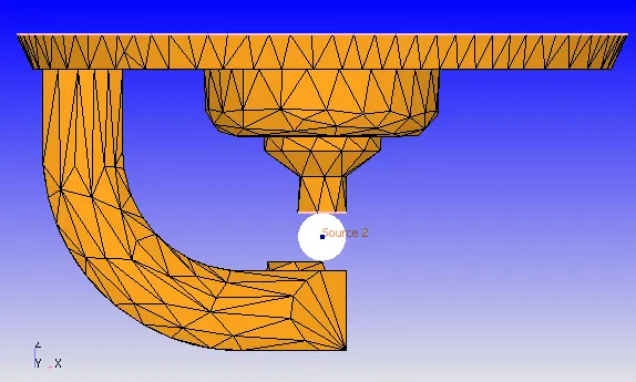
It is seen that the energy source is created in between spark end and spark plug. As soon as the spark generates it starts diffusing in all direction. So, it might happen that due to large element size numerical diffusion, which results in accuracy loss. To avoid it let us refine the mesh near source by adding fixed embedding.

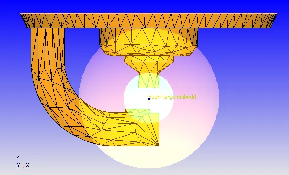
In above figure there are two fixed embedding provided. Embedding is set in shape of sphere whose center is same as that of energy source and it is valid for time of ignition i.e., -17 degrees to 8 degrees.

• There is option called injector embedding which provides embedding near injector.

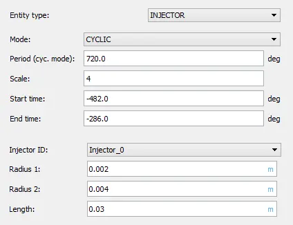
So, provide values as per above figure, provide start and end time for embedding, this time should be in range of time for fuel to be injected.

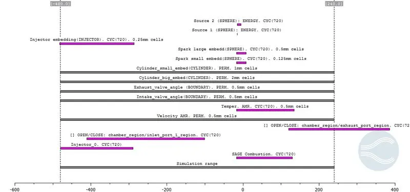• Now create output parameters and export input files for feeding in solver.
• Then validate case setup to check problems in setup, if find any resolve those problems.
• Then solve it using command line such as Cygwin.
• When simulation get over convert result files in to Parview VTK binary format to postprocess result data using Paraview.

Post processing:-

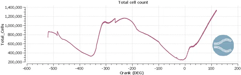The above figure is showing variation in number of cells with respect to degrees. Due to motion of components and embeddings the cell count is varying with time.

The cell count is depending on geometry primarily, as in CFD we mesh volume and in FEA we mesh solid component. In an IC engine which is in dynamic motion (continuously piston is moving up and down) the incylinder volume changes continuously. Hence number of cells are varying with crank angle in cylinder region. At intake stroke the fuel spray is injected in intake port and due to spray modelling the spray get divide in to small-small parcels which also vary cell count. In exhaust stroke as flue gases are emitting out of engine the number of cells at exhaust is also varying. Also, we have provided AMR and embedding to refine mesh at some locations. Embedding provided for particular time span refine mesh for only that particular time and due to that refinement cell count is increases. AMR is dependent on temperature and velocity which again refine mesh at some location. So overall effect of this cell count is always vary with respect to crank angle in simulation.

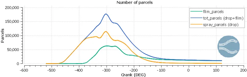The above plot shows number of parcels present at any time instant. The total number of parcels is addition of film parcel and drop parcels. After impinging on engine component's inner surface (cylinder surface, valve surface) the due to adhesive force some of spray drops are converted into film.

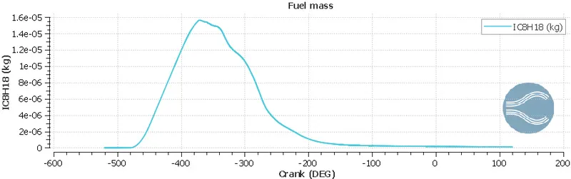The above plot shows mass of fuel at different instant. From above figure it is seen that in suction stroke the maximum amount of fuel is injected. From above figure the trapped fuel also can be calculated.

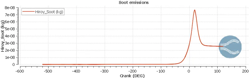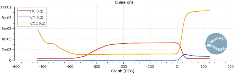
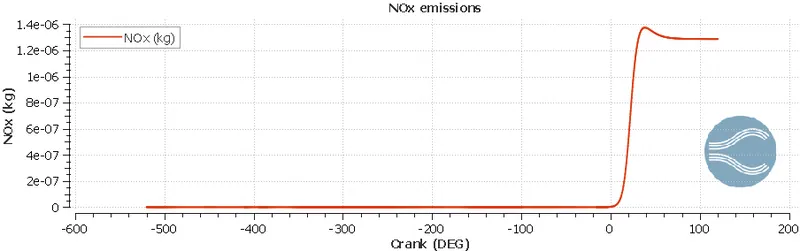
The above plots shows emission data with respect to time. It is seen from above plot that the carbon monoxide is presented in large amount due to incomplete combustion. This data can be used to benchmark the engine design and modifications.

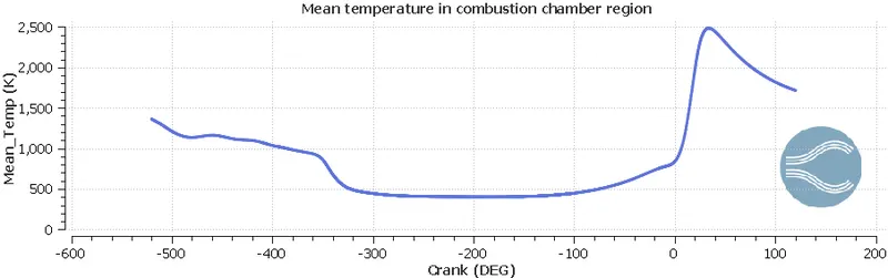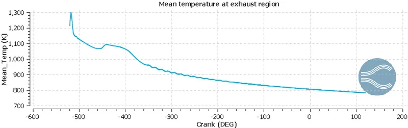Above plots shows temperature change in two different regions. The peak temperature in cylinder region shows spark is generated and due to high temperature spark combustion gets started inside combustion chamber. After combustion the exhaust gases also possess high temperature and it is seen in exhaust region plot.

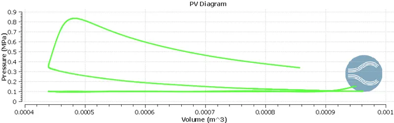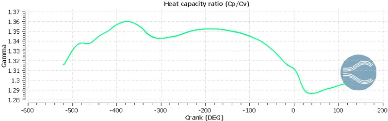The PV diagram is similar as Otto cycle which indirectly shows that our simulation setting is correct for SI engine. Gamma is ratio of specific heat at constant pressure to specific heat at constant volume, plotted over a time in second plot.

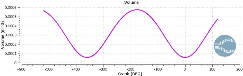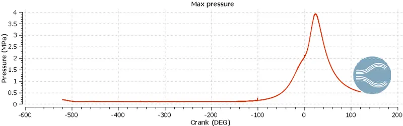
The above plot for pressure shows peak pressure generated, which is about 3.9 MPa. Due to expansion phase, it is seen that pressure is decreasing rapidly. In plot which is showing volume we can see the sinusoidal wave is present which is theoretically correct. The volume at BDC is about 0.000574m^3 and volume at TDC 5.703e-5.

Compression ratio: Compression ratio in an ICE is nothing but is nothing but degree to which the fuel mixture is compressed before ignition. It is defined as the maximum volume of the combustion chamber which obtained when the piston is farthest out means at bottom dead center divided by the volume with the piston in the full-compression position which is obtained when the piston at nearest of the cylinder head means at top dead center. Mathematically it can be given as-

`"Compression ratio"="Volume of cylinder when piston is at BDC"/"Volume of cylinder when piston is at TDC"`

`"Compression ratio"=(V_c+V_s)/V_c`

Where, Vc is Clearence volume

Vs is Swept volume

(Vc+Vs) is Total volume.

To compute compression ratio,

`CR = "Volume at BDC"/"Volume at TDC"= 0.000574/0.00005703`

`:.CR =10.065`

Swept volume is a volume travelled by piston and can be computed as-

`V_s = "Volume at BDC"-"Volume at TDC"`

`V_s= 0.000574-0.00005703=0.00051697m^3`

We have engine parameters as-

1. Bore =0.086 m
2. Stroke = 0.09 m

Swept volume using engine parameters can be computed as-

`V_s = pi/4xx"Bore"^2xx"Stroke length"`

`V_s = pi/4xx0.086^2xx0.09 = 0.0005228m^3`

And from this, it is seen that the swept volume from graph and from engine parameters are same, which indirectly shows that the compression ratio obtained is correct.

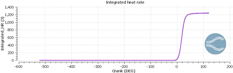From above plot it is visible that variation in integrated heat rate with respect to crank angle. The maximum integrated heat rate is 1241 J.

Combustion efficiency: Combustion efficiency is the rate at which an engine converts fuel into energy. We know that combustion efficiency is ratio of heat transferred in work to total heat theoretical heat generated by fuel. The term combustion efficiency can be mathematically driven by-

`eta_"combustion" = "Total heat released"/"Total heat of fuel"xx100`

Total heat released by fuel is nothing but integrated heat rate = 1241J.

Total heat of fuel = Mass of fuel X Calorific value of fuel

`:."Total heat of fuel" = (3xx10^-5)xx(44xx10^6) = 1320J`

To compute combustion efficiency-

`:.eta_"combustion" = 1241/1320 xx100= 94.01515%`

Volumetric Efficiency: Volumetric efficiency of an ICE is defined as the ratio of the mass density of the air fuel mixture drawn into the cylinder at atmospheric pressure to the mass density of the same volume of air in the intake manifold. It also denotes the ratio of air volume drawn into the cylinder to the cylinders swept volume.

Volumetric efficiency can be mathematically computed as-

`eta_"v"=V_a/V_s`

We have swept volume = 0.0005228 m^3

To compute air volume we have ideal gas equation,

`P.V_a=m.R.T`

Where,

`P="Atmospheric pressure of air"=101325N/m^2`

`R="Universal gas constant"=287J/(kg.k)`

`T="Temperature of air"=298.15K`

`m="Mass of air injected"`

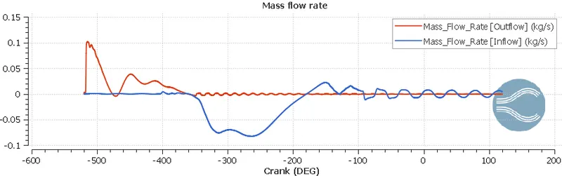
Mass can be computed from following plot-

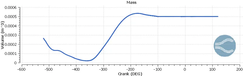
Hence, m = 0.0005348 Kg

Volume can be computed as-

`V_a=(m.R.T)/P=(0.0005348xx287xx298.15)/101325`

`V_a=4.5164e^-4 (m^3)`

`eta_"v"=4.5164e^-4/0.0005228=0.863885`

`:.eta_"v"=86.3885%`

In simple words, volumetric efficiency denotes the engine’s ability to carry out the work efficiently. Researchers try to improve the Volumetric Efficiency of an engine in many ways. However, this can be done most efficiently by compressing the incoming charge by using the forced induction method. Hence, the turbocharged/ Supercharged engines have more than 100% Volumetric Efficiency.

Air mass flow rate: As previously from graph we have seen that mass injected is 0.0005348 Kg.

For the 720 degrees we are injecting this 0.0005348 kg mass.

In our condition engine RPM are 3000, so if we wanted to convert it in RPS then,

`3000/60=50RPS`

Which means in 1 second 50-time crank is rotating.

Hence in 1 second crank is covering 50*360 = 18000 degrees.

Now let us calculate mass injected per second,

for 720 degrees => 0.0005348 kg

Then for 18000 degrees => x kg

`x=(18000xx0.0005348)/720 =0.01337 kg`

Hence, mass flow rate is 0.01337 kg/s

Engine performance calculator: It is the unique tool provided by Converge Science to compute engine performance.

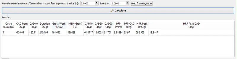The above figure shows outcomes for set engine parameters. The above results are obtained from engine performance calculator.

The terms CAD10, CAD50 and CAD90 gives crank angle at which 10, 50 and 90 percentage of fuel combust respectively. For ease of comparison, these values are relative to the start of the cycle.

CAD10 signifies that start of ignition or ignition lag, CAD50 indicates end of premixed combustion and phase change of fuel, CAD90 signifies that almost end of combustion.

CAD10 = 6.83717 Degrees

CAD50 = 18.4623 Degrees

CAD90 = 31.701 Degrees

Gross work = 468.646 Nm

Duration in degree = 240.199,

As we know, for 18000 degrees we need 1 seconds,

Then for 240.199 degrees we need to calculate time.

Hence, `240.199/18000=x/(1)`

`:.x=0.01334 Sec`

So power can be calculate as-

`Power="Work"/"Time"=468.646/0.01334`

`Power=35130J=35.13KJ`

`Power = (2piNT)/60`

`:.T=(35.13xx60)/(2pixx3000)=111.82Nm`

From the above paramters it is seen that combustion duration in degree is 240.2 so et us calculate it in seconds.

As we already calculated that in 1 second 18000 degrees are covered.

Hence for 240.2 Degrees time in second can be computed as-

`240.2/18000=0.01334 Sec`

Hence, combustion is remained for 0.01334 Seconds.

For performing IC engine simulation, we have to solve Navier Stokes equations, we need to model turbulence, combustion, spray droplet breakup, fuel mixing and fuel vaporization. So, it required very high computational cost to model all these sub-simulations simultaneously. Due to combustion, there is a temperature rise in combustion chamber, which results to increase in temperature of combustion chamber walls and it is necessary to compute that temperature to avoid system failure. Here CHT modelling comes in picture to help us in predicting wall temperature. Using CHT model with above IC engine model will consume high computational time and cost. So in such conditions to compensate computational cost wall heat transfer model is used.

Animations:-

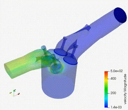
The above animation shows spray generation and spray propagation inside ICE. As per our modelling spray of fuel is injected through injector nozzles.

The above animation shows that how flame propagates and combustion takes place in combustion chamber. The animation generated is based on temperature. When high temperature spark generates through spark plug, the compressed charge (fuel + air mixture) inside cylinder starts burning and evenly propagate in cylinder.

Conclusion:-

1. Compression ratio for current case is 10.065.
2. Combustion efficiency obtained is 94%
3. Maximum torque obtained is 111.82 Nm.
4. Maximum power output obtained is 35.13KJ

References:-

1. Wikipedia
2. Britannica encyclopedia
3. Lagrangian CFD Modeling of Impinging Diesel Sprays
4. https://convergecfd.com/