Transient simulation of flow over a throttle body using Converge 3.0

Aim:-> To perform transient simulation of flow over throttle body.

Theory:-

In a traditional spark ignition gasoline engine, the throttle body is the part of the air intake system that controls the amount of air that flows into an engine's combustion chamber. It consists of a housing unit that contains a throttle plate (butterfly valve) that rotates on a shaft. Typically, it is located between the air filter and the intake manifold, the throttle body contains the delicate throttle system which controls air flow. The airflow helps to regulate the air-fuel mixture ratio required to ignite charge in an engine.

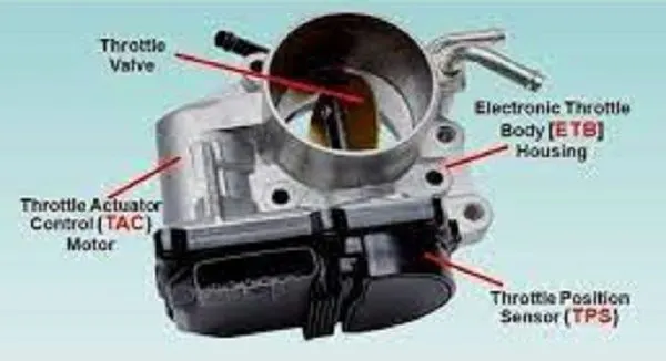Fig: Throttle body

The primary regulator for throttle pressure comes in the form of the throttle body temperature sensor, which measures the temperature of the air-fuel mixture entering the fuel injection system of vehicle. This necessary regulation helps spark ignitions generate the most fuel efficiency. The airflow is regulated by the driver via pressing on the acceleration pedal inside the vehicle. When the accelerator pedal is pushed down, the throttle plate (butterfly valve) opens and allows air into the engine. When the accelerator pedal is released, the butterfly valve (plate) closes and effectively chokes off (throttles) air flow into the combustion chamber. This process effectively controls the combustion rate inside the engine and ultimately the speed of the vehicle.

Butterfly valves are among the family of quarter-turn valves and work very similar to ball valves. The “butterfly” is a disk connected to a rod. It has a relatively simple construction which is shown in below image.

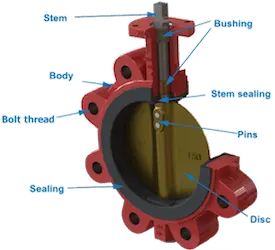Fig: Anatomy of Butterfly valve

The main components of a butterfly valve are the body, seal, disc and stem. A typical butterfly valve has the disc positioned in the center of the connected pipe and a stem that is connected to an actuator or handle on the outside of the valve. In the closed position, the disc is perpendicular to the flow to stop flow and it is sealed by the valve seat to restrict any leakages. The stem is also sealed by the use of an O - ring. When the actuator or handle rotates the stem back 90 degrees, the disc moves away from the valve seat and positions itself parallel to the flow. Partial rotation allows for the flow to be throttled or proportional.

Butterfly valves can come in diverse designs, each of which serve specific applications and pressure ranges. Butterfly valves can be categorized based on their disc closure design, connection design and actuation method as shown below.

• Disc closure design
  • Concentric
  • Eccentric
• Connection design
  • Wafer style
  • Lug style
• Actuation method
  • Manual Actuation
    • Hand lever
    • Gear
  • Automatic actuation
    • Electric
    • Pneumatic
    • Hydraulic

~Pre-processing:-

Geometry:-

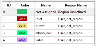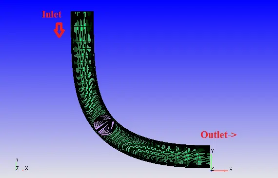
Fig: Geometry	Fig: Boundary flagging

In the above geometry of figure, the fluid enters through inlet in '-ve' Y direction and flows out through outlet in '+ve' X direction. The fluid is considered as air (`O_2:N_2 = 0.23:0.77`) for simulation purpose. The inlet pressure is 1.5 Bar and outlet pressure is 1 Bar. So due to pressure difference the fluid flows from inlet to outlet as per basic physics rule.

In adjacent figure the boundary flagging (defining boundary) is shown, the different color denotes different boundary in geometry. There are 4 boundaries considered in simulation.

Mesh:->

Fig: Meshed geometry preview	Fig: Enhanced view
Fig: Cell count and cell distribution for processing core

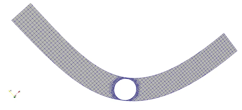
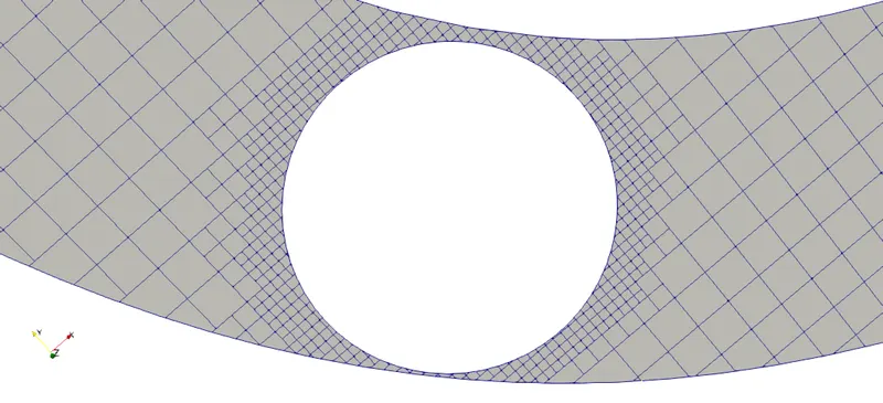
The mesh contour shows discretized geometry with particular element size like 0.002m. While setting up case we have provided fixed embedding of scale 2 and of 3 layers at valve, it results fine meshing near (around) valve. Providing embedding helps us to understand near wall phenomenon more precisely due to presence of complete and small mesh elements near valve.

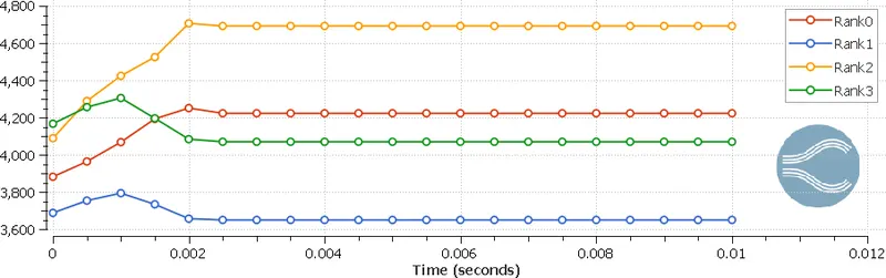
The plot with title of cell count shows number of cells processed during simulation by single processor. As we are using 4 cores so rank 0 denotes 1st core and rank 3 denotes 4th core. It is visible that for transient simulation the number of mesh elements are fluctuating till 0.002 seconds and then becoming stable, this happens due to dynamic meshing. As we know converge uses cut cell meshing technique and embedding allows similar geometry meshing near provided boundary. So here we have provided embedding for valve which and valve is rotating so embedding try to capture geometry at every time step and update mesh as per shape. This results fluctuations in mesh counts at every timestep. Total number of mesh elements in geometry can be calculated using addition of all cells in plot i.e., addition of cell by rank 0 to rank 3.

~Problem setting:-

Simulation parameters:-

• Type of simulation: Transient state
• Solver: Pressure based solver
• Mode: Full hydrodynamics
• Start time: 0 Seconds
• End time: 0.01 seconds
• Turbulence model: RNG K-epsilon
• Base grid: dx=dy=dz=0.002m

How to obtain end time of simulation?

Ans: As we know

`"Simulation time"=("Length of elbow")/("Flow velocity")`

As per steady state simulation the average velocity at outlet is 150m/s.

To calculate maximum elbow distance let us consider bounding box.

So Y=0.12m and X=0.106m.

Hence to find out maximum length of elbow, consider elbow as perfectly perpendicular means length of elbow is Y+X = 0.12+0.106 = 0.226m. The actual length of elbow must be less than 0.226m.

So time = 0.226/150 = 0.0015 seconds.

So fluid need 0.0015 seconds at most to reach at outlet.

And for simulation purpose lets take 5 to 7 times time to observe physics. So 0.01 Second is considered as simulation time.

Initial and boundary conditions:-

• Inlet: (Bound_id_1)
  • Boundary type: Inflow
  • Pressure = 1.5 Bar
  • Temperature = 300k
  • Species = Air

• Outlet: (Bound_id_2)
  • Boundary type: Outflow
  • Pressure = 1 Bar
  • Temperature = 300k
  • Species = Air

• Elbow_wall:
  • Boundary type: Wall
  • Law of wall

• Valve:
  • Boundary type: Wall
  • No slip
  • Surface movement: Moving
  • Wall motion: Rotating
    • Rotating center: (-0.0761534, 0.0390776, 0.0201742)
    • Rotation about: (0.794354, 0.607455, 0.000332307)

~Post-processing:-

Fig: Velocity contour

Fig: Plot showing average velocity at inlet and outlet at various time

Fig: Pressure contour

Fig: Plot showing static pressure at inlet and outlet at various time

Fig: Velocity stream vectors near valve

Fig: Plot showing mass flow rate at inlet and outlet at various time

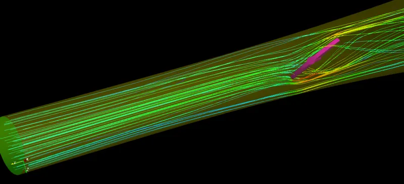Fig: Velocity streamlines

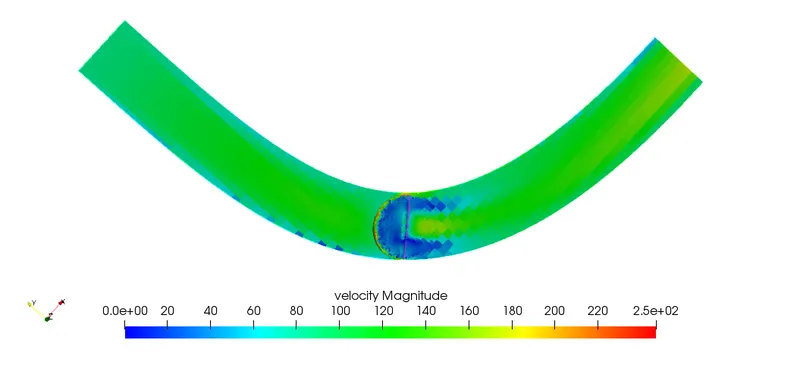
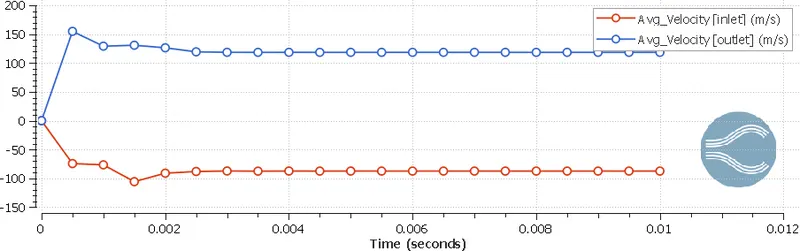
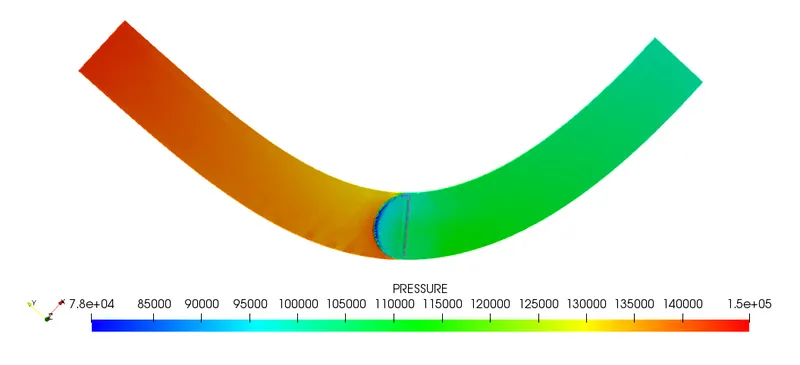
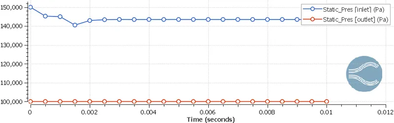
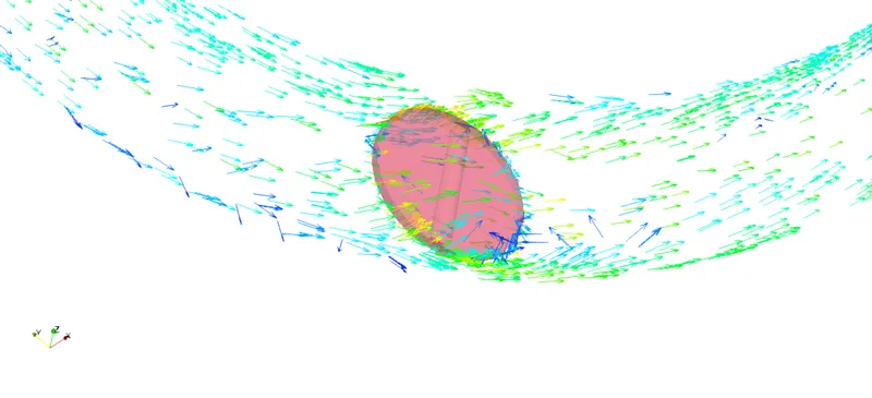
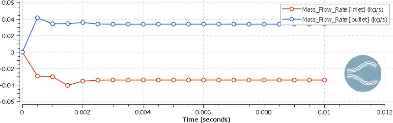
The above postprocessed data is self explaining. The pressure and velocity contours showing pressure and velocity at every mesh element, the lowest value is denoted in blue color and highest value is shown in red color for contours. When plots of velocity, pressure and mass flow rate are observed, at initial fluctuations in values is visible, after some time the fluctuations in curve damps down and became stable. This phenomenon shows that we are getting converged solution. The mass flow rate plot shows that 0.035kg/s fluid entering in system and leaving 0.035kg/s i.e., mass flow rate at inlet and outlet is equal which indirectly shows that law of conservation of mass is obeyed by fluid.

The pressure and velocity contours show high and low pressure and velocity positions. At initial the throttle valve is in open position so maximum amount of fluid is passing through it but as time increasing the valve is rotating. At 0.002 seconds valve is inclined at 25 degrees and remains stable in same position till end of simulation. Valve is present between way of flow hence, the flow gets restricted by valve body so fluid with high initial pressure is striking on valve which results high pressure at front of valve and this phenomenon is visible in pressure contour. In inlet and outlet velocity plot it is seen that at outlet fluid flows with up to 150m/s velocity. Due to 0.5 bar of pressure difference the fluid is attaining 150m/s speed.

Velocity animation:-

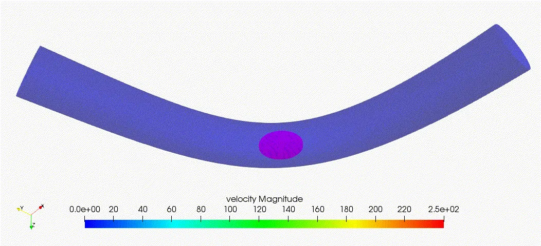
The above animation shows velocity flow in throttle body. The throttle valve is in open condition i.e., valve is parallel to flow of fluid which allows fluid to flow over valve. Providing embedding near valve results to visualize smooth flow in animation.

Throttle movement and dynamic mesh animation:-

To obtain following simulation we have used transient solver settings with no hydro dynamic mode. No hydrodynamic mode allows user to model and simulate dynamic mesh only. While solving no hydrodynamic simulation fluid transport equations which shows fluid behavior are kept disable by program itself, which allows user to simulate in less computational cost.

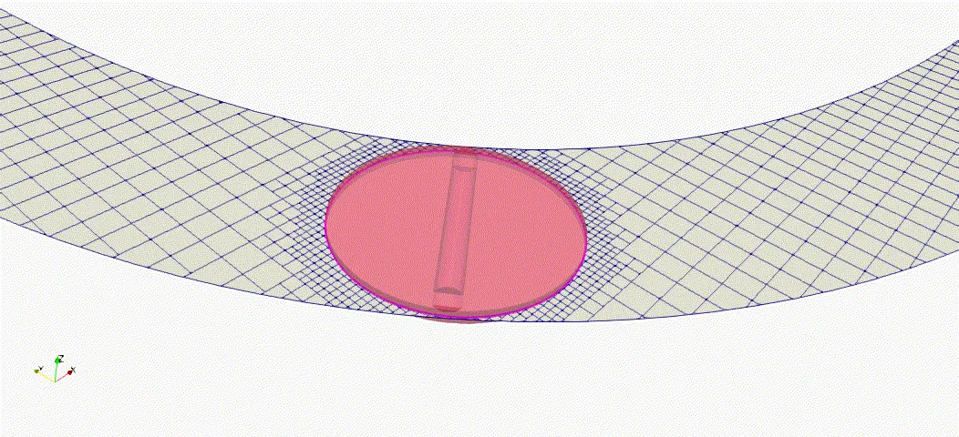
After observing above animation, it is seen that the throttle valve is rotating in a small amount (25 degrees) about central axis of cylinder and then getting stable. Here we have restricted rotation at 25 degrees for 0.002 seconds and our simulation end time is 0.01 second, so for last 0.008 seconds the valve is at stable position with inclination of 25 degrees.

Conclusion:- By observing postprocessed data it can be concluded that

1. Throttle body has important role in ICE.
2. Providing embedding increases accuracy of solution.
3. Steady simulation needs less computational cost than transient simulation.
4. Using no hydrodynamics allows us to check mesh generation process only.
5. To obtain more smooth animations, writing time interval of output file must be less