Rayleigh Taylor Instability phenomenon

Aim:-> To understand Phenomenon of Rayleigh Taylor instability using simulation on ANSYS fluent.

Theory:-

When a heavy fluid is kept over a light fluid under a gravity or under an external acceleration of the fluid system in the direction toward the denser fluid, the fluid interface becomes unstable. Such disturbance in interface tends to grow with time, producing the phenomena known as the Rayleigh–Taylor instability. The Rayleigh–Taylor instability for a fluid in a gravitational field was originally introduced by Rayleigh and later applied to all accelerated fluids by Taylor. This instability has been applied to a wide range of problems in CFD domain. The instability evolution would be too fast for direct observation.

An overview on characteristic flow patterns in the evolution of RT instabilities is given by the following figure. In this figure, the heavy fluid is represented by shaded (dark grayish) region and light fluid is represented by unshaded region and the gravitational acceleration is directed vertically downwards. The instabilities can be grouped in three types, mushroom formation, bubble formation i.e. rising structures formation and spikes creation i.e. falling structure formation.

Fig:- Rayleigh Taylor instability at various timestep

-Practical CFD models:-

SINGLE FLUID MODEL-

For above model there are 5 equations required. The equation consists of mass, momentum and energy equations for fluid mixture and two equations describes formation and growth of liquid phase.

It consist of following models-

1) Buoyancy drag model

2) Bensard Harlow Rauenzahn model

3) Potential flow model

TWO FLUID MODEL-

In above model we have separate set of governing equation i.e. mass, momentum and energy for vapor and liquid phases. In this model slip between vapor and liquid phase is considered. The two fluid model is most simplest case in multiphase model.

MULTIPHASE MODEL-

1. Volume of Fluid (VOF): Predicts the interface shape between immiscible fluid phases.
2. Discrete Phase Model (DPM): Particle interactions are neglected and the dispersed second phase occupies a low volume fraction (<10%). Population balance models are used to account for particle distributions.
3. Discrete Element Method (DEM): Tracks individual interacting particles. Used for flows with a high volume fraction of particles, where particle-particle interaction is important. Interaction with the fluid flow may or may not be important.
4. Eulerian Multiphase (EMO): Accurately models multiple separate, yet interacting, phases including liquids, gases or solids in any combination.
5. Euler-Lagrangian: Tracks the movement of individual droplets, bubbles or particles through continuous fluid phases to model the overall behavior. The particles typically occupy a small part of the total volume.
6. Eulerian-Eulerian Model (EEM): Models droplets, bubbles or particles dispersed in a continuous fluid phase. The dispersed particles act as a continuum and are not tracked individually.
7. Eulerian-Granular Model (EGM): Uses Eulerian approach to model dispersed particles in a continuous fluid. Uniform-sized particle motion is modeled using averages, not individually. In this model both particle-wall and particle-particle interaction are considered.

Simulation:-

The analysis is done for 3 different mesh sizes. As analysis consist of two fluids so multi fluid model is considered, and VOF method is used.

Geometry:-

Above figure represents geometry setup for simulation. Here for computational memory optimization we are performing surface i.e. 2D simulation. As we know in case of Rayleigh Taylor instability the fluid with higher density is superimposed on fluid with low density. Hence as per above condition we have set up geometry.

Meshing:-

Fig:- Meshed geometry

Above figure shows meshed geometry. We have considered three mesh sizes to compare the effect of mesh size on simulation and results. Above figure shows refined meshed geometry.

Solver and initial conditions:-

For solving this type of simulation we need to used transient method only. Because steady state simulations are better in case of visualization of result at final state or equilibrium state. But in our case of Rayleigh Taylor instability, we have more focus on irregularities developing at various timesteps. In case of transient simulation only it is possible to capture bubbles, vortices, shockwaves and behavior of fluid at every instances in model. That's why for such conditions transient method is better than steady state method.

CASE SETUP:

• Pressure based solver is considered
• Transient state method is used
• Gravity is enabled in negative Y direction
• Viscus laminar model is chosen
• Multiphase model with volume of fluid is considered for two Eulerian phases, and select implicit scheme.
• Patching of the volume fraction of the two phases is performed before the start of simulation. Phase used for patching was water and volume fraction of 1 is taken for water surface and 0 for air surface.

Fig:- Initial condition for simulation

Above figure shows volume fraction of fluid at initial time t=0Seconds. The red color shows water and blue shows air.

~Case A (Baseline mesh):-

Mesh size = 0.5mm

Number of nodes = 3321

Number of elements = 3200

Fig:- Residual V/S iteration plot

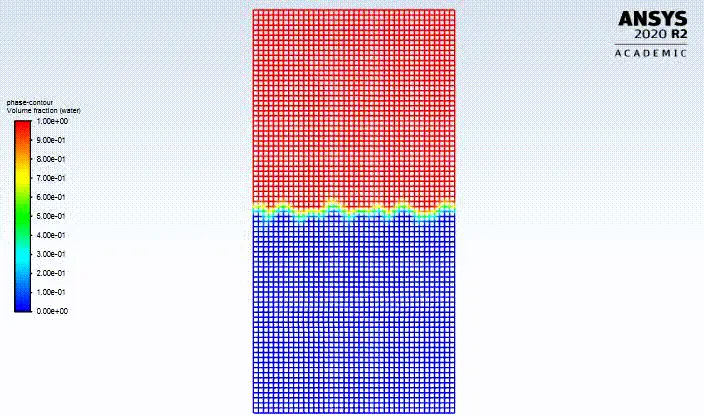Fig:- Phase animation

~Case B:-

Mesh size = 0.35mm

Number of nodes = 6670

Number of elements = 6498

Fig:- Residual V/S iteration plot

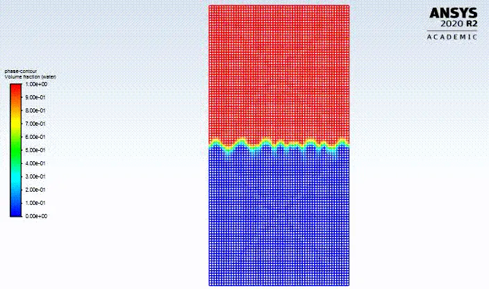Fig:- Phase animation

~Case C:-

Mesh size = 0.25mm

Number of nodes = 13041

Number of elements = 12800

Fig:- Residual V/S iteration plot

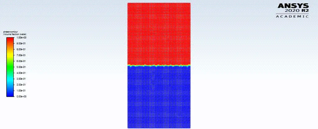Fig:- Phase animation

~Case D (For user defined material & water):-

Mesh size = 0.25mm

Number of nodes = 13041

Number of elements = 12800

In this case we have considered user defined material as a low density material instead of air. The properties for defined material are as follows-

Density = 400 kg/m³,

Viscosity = 0.001 kg/m-s

Fig:- Residual V/S iteration plot

Fig:- Phase animation

Atwood number:-

It is a non dimensional number used in fluid dynamics, it is important parameter in study of hydrodynamic instabilities in density stratified flow. It is dimensionless density ratio and computed as-

`A=(rho_a-rho_b)/(rho_a+rho_b)`

Where,

`rho_a=` density of heavier fluid

`rho_b=` density of lighter fluid

1st case-

Fluid material are water and air

Density of water (heavy fluid) = 998 kg/m^3

Density of air (light fluid) = 1.225 kg/m^3

Hence Atwood number,

`A=(998-1.225)/(998+1.225)=0.99755`

Atwood number = 0.99755

2nd case-

Fluid material are water and user defined material

Density of water (heavy fluid) = 998 kg/m^3

Density of user defined material (light fluid) = 400 kg/m^3

Hence Atwood number,

`A=(998-400)/(998+400)=0.42775`

Atwood number = 0.42775

Variation in Atwood number affects behavior of instability.

For the case of smaller Atwood Number, the density difference between the two sides of the interface is small and the density distribution of the upper and lower layers is nearly symmetrical. The initial density stratification plays a dominant role and the expansion compression effect has a little influence. With the increased Atwood Number close to 1 the stabilization effect of initial density stratification decreases and the instability caused by the expansion-compression effect becomes more significant. It is observed that with larger Atwood Number, larger amplitude of perturbations exists. It is due to the larger density ratio of the two fluids, the stronger is the force to develop the interface instability.

Atwood number is important parameter in RTI analysis, the penetration distance of heavy bubble fluid into light fluid can be computed by-

`Axxgxxt^2`

Where,

g = Acceleration due to gravity,

t = time

A = Atwood number.

Conclusion:-

1. Instability is quite fast for large Atwood number (close to 1).
2. With decreased in mesh size we get perfect mixing and instabilities in model.
3. For refined mesh the visualization of solution animation is good, precise and smooth but it takes more time and iterations to settle down heavy liquid at bottom.
4. Transient analysis is necessary to capture perfect mixing behavior of fluid.
5. To avoid floating error we need to choose timestep wisely.