1D Combustion flame-speed simulation for Methane and Hydrogen combustion using Python & Cantera

Aim:-> To perform 1D combustion flame speed analysis using Cantera and Python coding.

Theory:-

Flame:

Flame word is originated from Latin word 'flamma'. A flame is the visible gaseous part of fire generated due to exothermic reaction in very small area. The flame occupies a small portion of the combustible mixture at any one time and it is propagating towards the unburnt gases.

Premixed flames occurs in any homogeneous mixture where the fuel and oxidant are mixed prior to reaction. Such premixed flames can progress either as deflagration or detonation process means the combustion wave can be travelled sub-sonically or super-sonically, the subsonic wave is called as deflagration and supersonically travelled wave can termed as detonation. In real world the combustion happens in 3D, there is nothing like 1D combustion. But for simulation purpose and simplicity we need to assume that flame is flat along cross section of combustion chamber and propagate only in single direction (flame propagates in one direction and in all other directions it is homogeneous).

Flame speed:

It is the measure of expansion of flame front after ignition (the rate at which the unburnt mixture is entering the flame). Flame speed represents how rapidly the flame travels from an absolute reference point, while burning velocity signifies the moving rate of chemical reactants i.e. unburned gases into the flame front from a local reference point located on the flame front. Flame speed is emphasized because it is the property which dictates flame shape and important flame characteristics like blowoff and flashback. The flame speed could be either laminar or turbulent by nature which is depended on the velocity of the unburned charge particles. Various approaches are used for simulation flame velocity, which includes either heat diffusion or mass diffusion while some of theories consider equal importance to both effects.

In general (real world) the flame speed simulation is transient in nature. But by using flame reference co-ordinates it can be customized into steady state simulation. So we need to fix the origin at the flame front and as the flame moves the coordinates moves simultaneously. Thus, the simulation becomes a steady state problem cause both points moves simultaneously. As steady state simulation is cheap and saves computational time, hence most of the time user prefers steady simulation approach to simulate combustion flame speed.

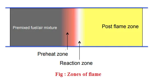
It is convenient to divide the flame in different zones such as:

1. Premixed charge:
   • Mixture of air and fuel present
2. Preheat zone:
   • Little heat is released
   • Heating of reactant
3. Reaction zone:
   • Bulk of chemical energy is released
   • Fuel gets decomposed
   • High temperature zone
   • Generally thin as compared to pre-heat zone
4. Post flame zone:
   • Hot products after combustion are present
   • NOx formation

While performing flame speed simulation we need to assume that-

• The simulation is 1D in nature
• Mach number is very low for flame
• Mechanical energies, viscous dissipation and pressure difference across the flame front are negligible
• The specific heat capacity, thermal conductivity and thermal diffusivity are constant across the flame front
• Flame is thin means it consists high activation energy
• Unburnt particles entered into flame front, got combust and leave from flame front as a burned product
• Lewis number is unity (Le = 1)
• Steady-state conditions which means a spatially stationary flame front is considered

The stochiometric combustion reaction for methane can be given as follows:

`CH_4 + 2(O_2 + 3.76N_2)<=>CO_2 + 2H_2O +7.52N_2`

The stochiometric combustion reaction for hydrogen can be given as follows:

`2H_2 + O_2 +3.76N_2<=>2H_2O+3.76N_2`

As we know Cantera needs chemical reaction mechanism files to find out NACA polynomials values and to calculate required functions value. This mechanism has been developed to describe flame propagation, flame structure, and ignition phenomena. So "GRI 3.0.cti" is basically designed for combustion of hydrocarbons. It is possible to use same file for hydrogen combustion simulation, but using it will give less accurate result and also may consume more time to converge. So for hydrogen combustion we have introduced separate ".cti" file in code. The Hydrogen mechanism is developed in 2004, which properly simulates laminar flame speeds, flame compositions, and shock tube ignition delay times for hydrogen combustion reaction and also reduce computation time.

Python code for computing flame speed:

'''
Program to copute flame speed for combustion flames

Methane combustion reaction:
CH4 + 2(O2 + 3.76N2) <-> CO2 + 2H2O + 7.52N2

Hydrogen combustion reaction:
2H2 + (O2 + 3.76N2) <-> 2H2O + 7.52N2

'''

# Importing libraries
import cantera as ct 
import matplotlib.pyplot as plt 
import numpy as np 

# Creating gas instance
gas_m = ct.Solution('gri30.cti','gri30_mix') # This instance is for methane reaction
gas_h = ct.Solution('H2_mech.cti') # This instance is for hydrogen reaction

# Initial temperature in K
T = 300

# Initial pressure in atm
P = ct.one_atm

# Reactant compositions
## For methane (Here we have consider lean mixture)
Reactants_m = 'CH4:0.45, O2:1, N2:3.76'
## For hydrogen
Reactants_h = 'H2:2, O2:1, N2:3.76' 

# Introducing initial condition to reactor object
gas_m.TPX = T, P, Reactants_m
gas_h.TPX = T, P, Reactants_h

# Width of flame in m
w = 0.03

# For Methane combustion
## Applying freeflame condition for flame speed
f = ct.FreeFlame(gas_m, width=w)
## Setting refining parameter to curve
f.set_refine_criteria(ratio=2, slope=0.07, curve=0.14)

# For Hydrogen combustion
## Applying freeflame condition for flame speed
g = ct.FreeFlame(gas_h, width=w)
## Setting refining parameter to curve
g.set_refine_criteria(ratio=2, slope=0.07, curve=0.14)

# Solving
f.solve()
g.solve()

# Printing flame speeds
print('Flamespeed for Methane flame = {:7f} m/s'.format(f.u[0]))
print('Max temperature for Methane flame = {:7f} k'.format(max(f.T)))
print('Flamespeed for Hydrogen flame = {:7f} m/s'.format(g.u[0]))
print('Max temperature for Hydrogen flame = {:7f} k'.format(max(g.T)))
#help(f)

# Concentration and mole fraction of CO2
conc_m_CO2 = f.concentrations[gas_m.species_index('CO2'), :]
Mole_fraction_m_CO2 = f.X[gas_m.species_index('CO2'), :]
conc_h_CO2 = g.concentrations[gas_h.species_index('CO2'), :]
Mole_fraction_h_CO2 = g.X[gas_h.species_index('CO2'), :]

# Plotting
## For methane combustion
plt.figure(1)
plt.subplot(2,1,1)
plt.plot(f.grid,f.T,color='purple',linewidth=2)
plt.xlabel('Width of flame',fontweight='bold')
plt.ylabel('Temperature [$k$]',fontweight='bold')
plt.grid('both',linestyle='--',linewidth=0.8)
plt.subplot(2,1,2)
plt.plot(f.grid,f.u,color='red',linewidth=2)
plt.xlabel('Width of flame',fontweight='bold')
plt.ylabel('Flame-speed [$m/s$]',fontweight='bold')
plt.grid('both',linestyle='--',linewidth=0.8)

plt.suptitle("For combustion of Methane with width "+str(w),fontweight='bold')
plt.tight_layout()

plt.figure(2)
plt.subplot(2,1,1)
plt.plot(f.grid,conc_m_CO2,color='blue',linewidth=2)
plt.xlabel('Width of flame',fontweight='bold')
plt.ylabel('Concentration of CO2',fontweight='bold')
plt.grid('both',linestyle='--',linewidth=0.8)
plt.subplot(2,1,2)
plt.plot(f.grid,Mole_fraction_m_CO2,color='magenta',linewidth=2)
plt.xlabel('Width of flame',fontweight='bold')
plt.ylabel('Mole fraction of CO2',fontweight='bold')
plt.grid('both',linestyle='--',linewidth=0.8)

plt.suptitle("Variation of CO2 for Methane combustion at width "+str(w),fontweight='bold')
plt.tight_layout()

## For hydrogen combustion
plt.figure(3)
plt.subplot(2,1,1)
plt.plot(g.grid,g.T,color='purple',linewidth=2)
plt.xlabel('Width of flame',fontweight='bold')
plt.ylabel('Temperature [$k$]',fontweight='bold')
plt.grid('both',linestyle='--',linewidth=0.8)
plt.subplot(2,1,2)
plt.plot(g.grid,g.u,color='red',linewidth=2)
plt.xlabel('Width of flame',fontweight='bold')
plt.ylabel('Flame-speed [$m/s$]',fontweight='bold')
plt.grid('both',linestyle='--',linewidth=0.8)

plt.suptitle("For combustion of Hydrogen with width "+str(w),fontweight='bold')
plt.tight_layout()

plt.figure(4)
plt.subplot(2,1,1)
plt.plot(g.grid,conc_h_CO2,color='blue',linewidth=2)
plt.xlabel('Width of flame',fontweight='bold')
plt.ylabel('Concentration of CO2',fontweight='bold')
plt.grid('both',linestyle='--',linewidth=0.8)
plt.subplot(2,1,2)
plt.plot(g.grid,Mole_fraction_h_CO2,color='magenta',linewidth=2)
plt.xlabel('Width of flame',fontweight='bold')
plt.ylabel('Mole fraction of CO2',fontweight='bold')
plt.grid('both',linestyle='--',linewidth=0.8)

plt.suptitle("Variation of CO2 for Hydrogen combustion at width "+str(w),fontweight='bold')
plt.tight_layout()

plt.show()

Output obtained from above code:

Flamespeed for Methane flame = 0.336805 m/s
Max temperature for Methane flame = 2137.867001 k
Flamespeed for Hydrogen flame = 2.421423 m/s
Max temperature for Hydrogen flame = 2372.994155 k

Output plots obtained:

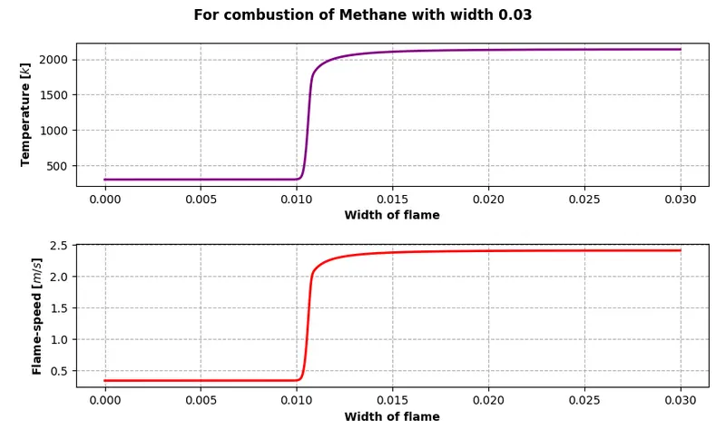Fig 1: For Methane combustion reaction

Since the flame heats the products, the product density is less than reactant density. As per continuity equation the burn gas velocity will be greater than velocity of unburnt gas and it is visible in plots.

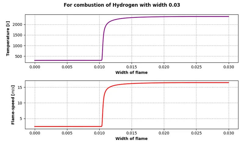Fig 2: For Hydrogen combustion reaction

The above figures (fig 1 & fig 2) show plots of variation of variables such as temperature and velocity along the length of the domain (Width). The width of domain is considered as 0.03m for above case. The flame propagation starts from origin i.e. from X = 0. From this origin the unburnt charge (mixture of air and fuel) enters the flame. The unburnt charge is possess properties of initial condition i.e. temperature of 300k and pressure of 1atm. As the unburnt charge particles move into the flame, the combustion reaction occurs which effects to increase in flame temperature. At a certain point we can see the sudden peak in the temperature and velocity which denotes that ignition is takes place and most of the unburnt charge converted into product.

Fuel	Flame speed (m/s)	Max temperature (k)	Number of grid points
Methane	0.336805	2137.867001	160
Hydrogen	2.421423	2372.994155	132

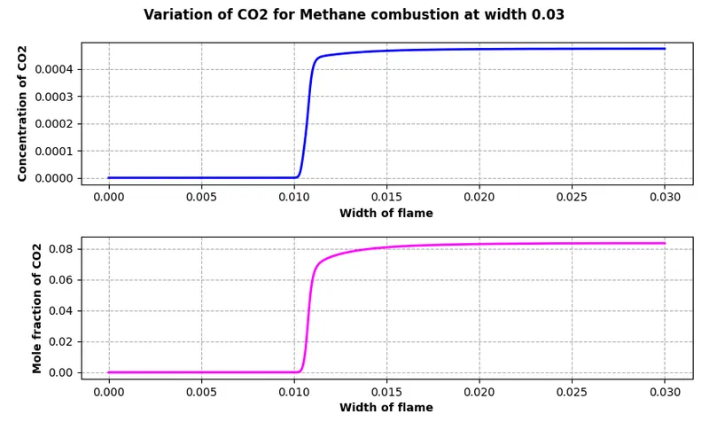
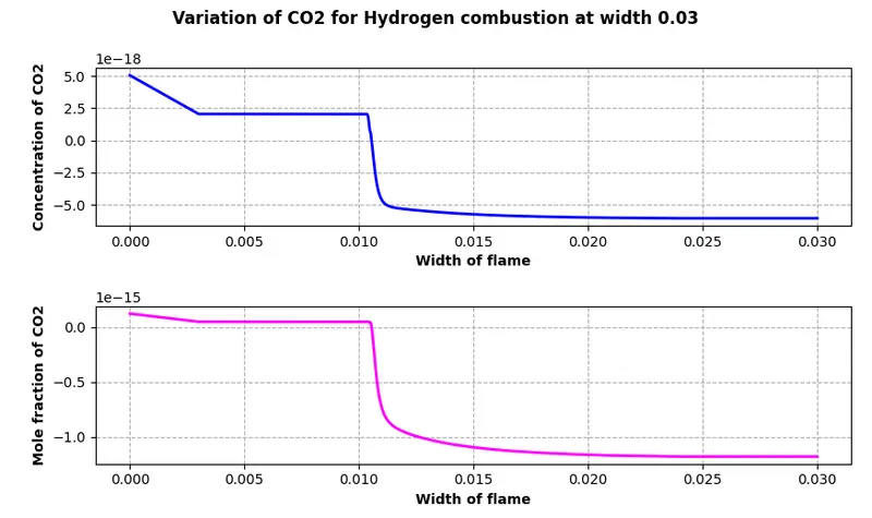
To compute mole fractions and concentration the following commands are used:

• To compute the mole fractions:- `" f.X[gas_m.species_index('CO2'), :]"`
• To compute concentration:- `" f.concentrations[gas_m.species_index('CO2'), :]"`

# Concentration and mole fraction of CO2
conc_m_CO2 = f.concentrations[gas_m.species_index('CO2'), :]
Mole_fraction_m_CO2 = f.X[gas_m.species_index('CO2'), :]
conc_h_CO2 = g.concentrations[gas_h.species_index('CO2'), :]
Mole_fraction_h_CO2 = g.X[gas_h.species_index('CO2'), :]

It can be seen from the above plots that there is an increase in CO2 concentration for methane burning indicating the formation of CO2. But in case of hydrogen combustion there is negligible CO2 formation which is obvious due absence of carbon dioxide atom.

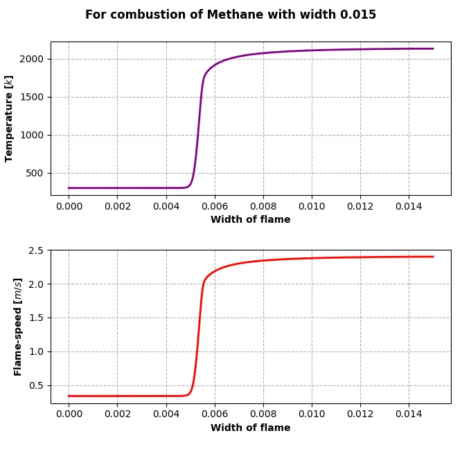
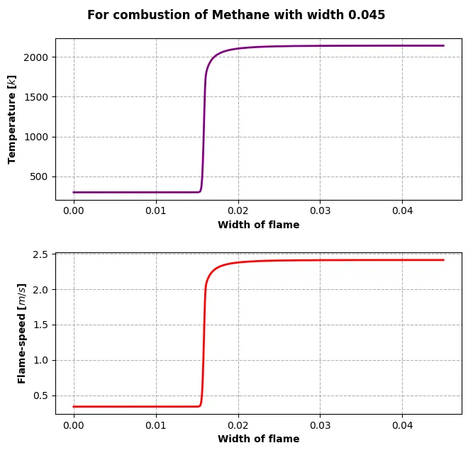
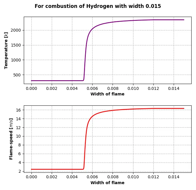
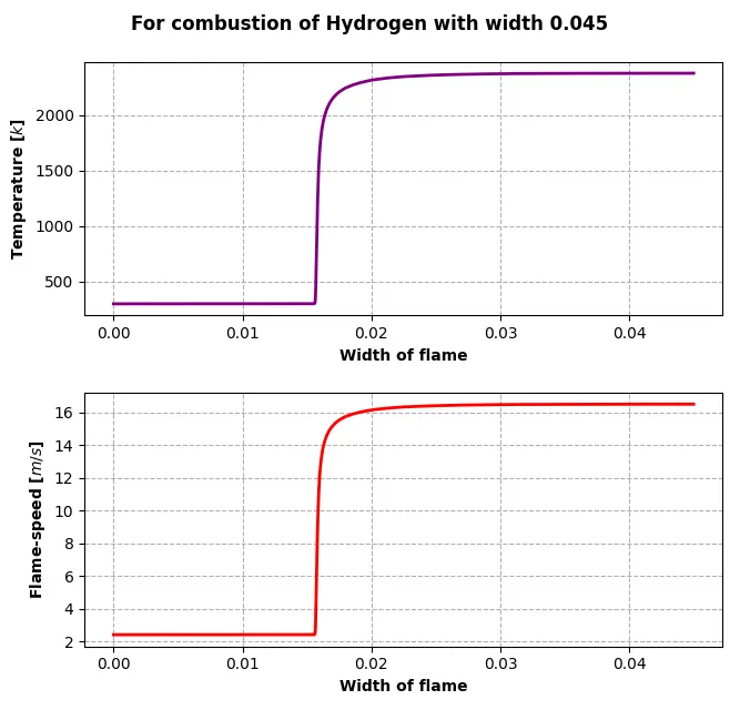
Flame width (w) = 0.015 m	Flame width (w) = 0.045 m
Output: Flamespeed for Methane flame = 0.336595 m/s Max temperature for Methane flame = 2130.849014 k Flamespeed for Hydrogen flame = 2.421504 m/s Max temperature for Hydrogen flame = 2347.963528 k	Output: Flamespeed for Methane flame = 0.337787 m/s Max temperature for Methane flame = 2138.829825 k Flamespeed for Hydrogen flame = 2.419805 m/s Max temperature for Hydrogen flame = 2377.875215 k
Table: Comparison for different flame width

The width parameter basically represents the length of the domain. The flame will travel along the length of this domain. When we change the width parameter value, it is seen that the number of nodes generated by Cantera are also varies and which directly influence computation time required for simulation. It’s visible from above plots that width parameter has effect on ignition. For width of 0.015m ignition is occurring at 0.005 and for width of 0.045m ignition is occurring at 0.015. But width parameter doesn’t show much variation in flame velocity.

Conclusion:- From observing above result data and plots it can be conclude that-

1. For combustion reaction of hydrogen it is necessary to import different ".cti" file which consist reactions mechanism for hydrogen. (Like in our simulation we have imported "H2_mech.cti" file)
2. Hydrogen combustion occurs more aggressively than the methane combustion.
3. It has been observed that the accuracy of the calculated flame speed is highly sensitive to the number of grid points used in the calculations.
4. The width parameter does not have a huge effect on the solution parameters like flame speed and maximum temperature as long as the domain is big enough for Cantera to perform the time-integration.
5. Choosing proper width for simulation is necessary because if the domain width is too small, the solution will not be able to converge properly.
6. Velocity and temperature of unburnt charge is less than burnt product.