Simulation of Prandtl-Meyer Shock problem at various sub-grid criterion
Aim:-> To simulate Prandalt Mayer shock wave problem at various sub grid criterion.
Theory:-
Shock wave:
A wave is a propagating dynamic disturbance (change from equilibrium) of one or more quantities. A shock wave or shock, is a type of propagating disturbance that moves faster than the local speed of sound in the medium. Similar as an ordinary wave, a shock wave carries energy and can propagate through a medium but is characterized by an abrupt, nearly discontinuous, change in pressure, temperature, and density of the medium. As the shock generates at velocity more than speed of sound hence it is observed only in supersonic flows and sonic flows not in subsonic flow. In a shock wave the properties of the change almost instantaneously.
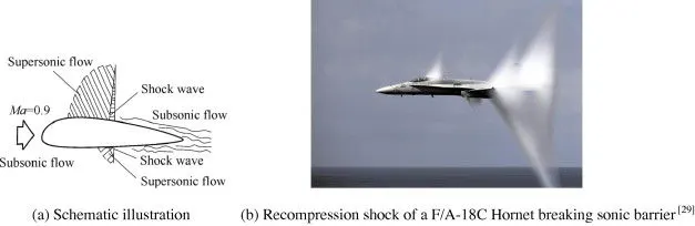 |
| Fig: Recompression shock wave |
As an object moves through a gas, the gas molecules are deflected around the object. The phenomenon can be divided in following three types.
- If the speed of the object is much less than the speed of sound of the gas, the density of the gas remains constant and the flow of gas can be described by conserving momentum and energy.
- As the speed of the objects increases towards the speed of sound, we must consider compressibility effects on the gas. The density of the gas varies locally as the gas is compressed by the object.
- When an object moves faster than the speed of sound, when a pressure front moves at supersonic speeds and pushes on the surrounding air. At the region where this occurs, sound waves travelling against the flow reach a point where they cannot travel any further upstream and the pressure progressively builds in that region; a high pressure shock wave rapidly forms. Or when there is an abrupt decrease in the flow area, shock waves are generated. If the flow area increases, however, a different flow phenomenon is observed.
Shock waves are not conventional sound waves; a shock wave takes the form of a very sharp change in the gas properties. Shock waves in air are heard as a loud "crack" or "snap" noise. Over longer distances, a shock wave can change from a nonlinear wave into a linear wave, degenerating into a conventional sound wave as it heats the air and loses energy.
Mach number and types of flows:
The Mach Number is a dimensionless value useful for analyzing fluid flow dynamics problems where compressibility is a significant factor. The Mach number can be expressed numerically as-
`M = v/c`
Where,
M = Mach number
v = Fluid flow velocity in m/s
c = Local speed of sound in m/s
On basis of Mach number flow can be classify in following types:-
|
Regime |
Subsonic |
Transonic |
Sonic |
Supersonic |
Hypersonic |
|
Mach Number |
< 0.8 |
0.8 – 1.3 |
1.0 |
1.3 – 5.0 |
5.0 – 10.0 |
Prandtl–Meyer expansion fan:
A supersonic expansion fan which is also called as Prandtl–Meyer expansion fan in technical terminology can be considered as a continuous sequence of infinitesimal Mach expansion wave. The wave is a two-dimensional simple wave and generated due to a centered expansion process that occurs when a supersonic flow turns around a convex corner. The fan consists of an infinite number of Mach waves, diverging from a sharp corner. When a flow turns around a smooth and circular corner, these waves can be extended backwards to meet at a point. Each wave in the expansion fan turns the flow gradually in small steps. It is physically impossible for the supersonic flow to turn through a single ‘shock wave’ because this would violate the second law of thermodynamics.
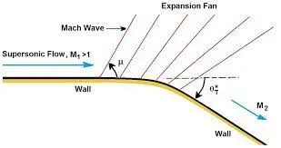 |
As mentioned above, the Mach number of a supersonic flow increases through an expansion fan. The amount of the increase depends on the incoming Mach number and the angle of the expansion. The physical interpretation of the Prandtl-Meyer function is that it is the angle through which you must expand a sonic (M=1) flow to obtain a given Mach number. The value of the Prandtl-Meyer function is therefore called the Prandtl-Meyer angle.
It is easy to find out differences between shock waves and expansion fans. Across a shock wave, the Mach number decreases, the static pressure increases, and there is a loss of total pressure because the process is irreversible. And for expansion fan the process is isentropic, the Mach number increases, the static pressure decreases and the total pressure remain constant, while the static pressure, temperature and density decreases.
Boundary conditions:
Boundary conditions are constraints for problem which are necessary for the solution of a boundary value problem. Boundary condition can be defined as a set of restriction condition provided to differential equation for limiting the possible solution. A boundary value problem includes a differential equation or system of differential equations to be solved in a domain on whose boundaries i.e., a set of conditions are known. Initial condition can be defined as an extra information that tells you the value of the function at a particular (initial) point in any differential equation. We need boundary conditions and initial conditions to solve differential equation and to obtained an unique solution.
Boundary value problems are exactly opposite to the initial value problem, in which only the conditions on one extreme of the interval are known. Boundary value problems are extremely important because by using such type of problems one can easily model many critical physics phenomena and applications, from solid mechanics to heat transfer, from fluid mechanics to acoustic diffusion. They arise naturally in every problem based on a differential equation to be solved in space, while initial value problems usually refer to problems to be solved in time.
Types of boundary conditions are as follows:
- Dirichlet
- Neumann
- Robin
- Mixed
- Cauchy
Boundary condition used for shock wave:
For problem to solve, the values of the variables like pressure, velocity and temperature are not available before solving the problem. As we know the pressure at the outlet boundary conditions requires the specification of static pressure. The value of the specified static pressure is used only while the flow is subsonic. If the flow is supersonic, the specified pressure will no longer be used. Hence none of value is specified at a supersonic outlet and all variables are extrapolated from the domain interior. So it is possible by using Neumann boundary conditions. So for the classic shock wave problems Neumann Boundary condition is used.
~Pre processing:-
Geometry:-
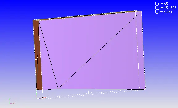 |
In the above geometry of figure, the fluid enters through inlet and flows out through outlet. Fluid flows in '+ve' X direction. The fluid is considered as air (`O_2:N_2 = 0.23:0.77`) for simulation purpose. Air through the inlet velocity of 2 Mach (680m/s) is entered in a domain, the inlet temperature is 286.1k and exit temperature 300k. As we have considered problem as 2D simulation so ignoring Z direction for problem.
~Problem setting:-
Simulation parameters:-
- Type of simulation: Steady state
- Solver: Pressure based solver
- Mode: Full hydrodynamics
- Start time: 0 Cycles
- End time: 20000 Cycles
- Time step: 1e-7
- Turbulence model: RNG K-epsilon
- Base grid: dx=dy=dz=0.8m
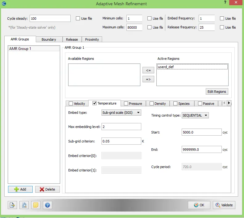
- Adaptive mesh refinement: Temperature based
- Active region:- User defined region
- Max. embedding level:- 2
- Sub-grid criterion:- 0.05 k
Initial and boundary conditions:-
- Inlet: (Bound_id_1)
- Boundary type: Inflow
- Velocity = 680 m/s
- Temperature = 286.1k
- Species = Air
- Outlet: (Bound_id_2)
- Boundary type: Outflow
- Pressure = Zero gradient
- Velocity = Zero gradient
- Temperature = 300k
- Species = Air
- Top and bottom wall:
- Boundary type: Wall
- Slip wall
- Front face:
- Boundary type: 2D
- Back face:
- Boundary type: 2D
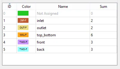 |
In above figure the boundary flagging (defining boundary) is shown, the different color denotes different boundary in geometry. There are 5 boundaries considered in simulation.
~Post-processing:-
Mesh details:-
| For SGC = 0.05k | For SGC = 0.01k |
 |
 |
| Fig: Mesh geometry | |
 |
 |
| Fig: Mesh enhanced view | |
 |
 |
| Fig: Cell count per processor | |
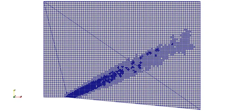
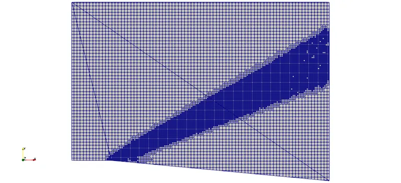
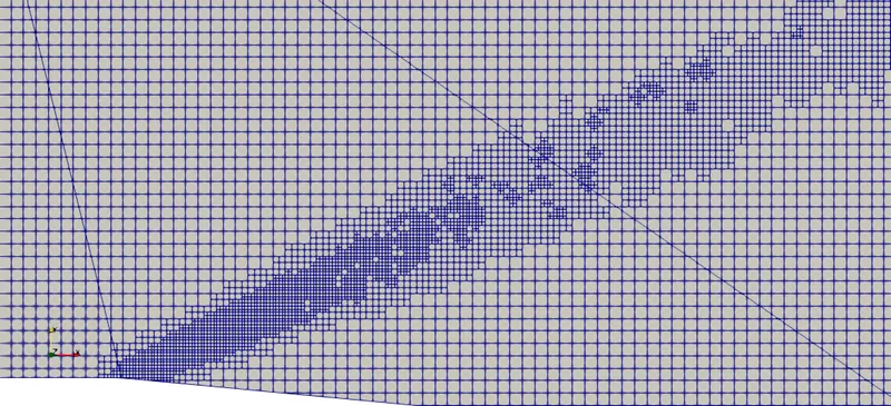
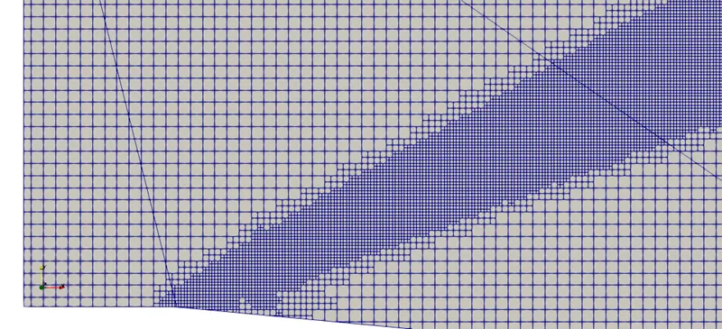
In the above mesh contour, discretized geometry with particular element size like 0.8m is shown. While setting up case we have provided adaptive mesh refinement of sub-grid criterion of 0.05 and 0.01 with maximum embedding of 2, it results fine meshing where the temperature change is below sub grid criterion. Providing embedding helps us to understand layer separation phenomenon more precisely due to presence of complete and small mesh elements.
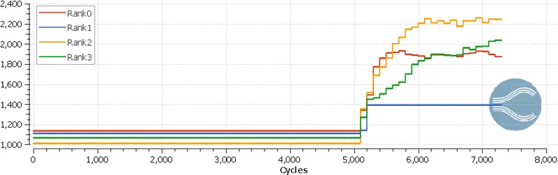
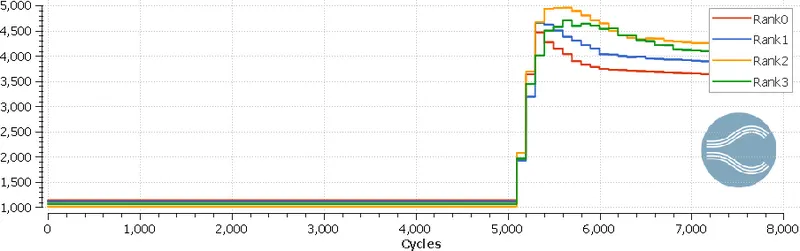
The plot with title of cell count shows number of cells processed during simulation by single processor. As we are using 4 cores here in simulation, so rank 0 denotes 1st core and rank 3 denotes 4th core. Total number of mesh elements in geometry can be calculated using addition of all cells in plot i.e., addition of cell by rank 0 to rank 3.
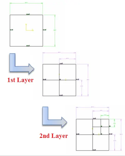
It is visible in cell count plot that after some time the cell count is increasing, the reason behind it is AMR. Adaptive Mesh Refinement (AMR) automatically adjusts the grid at each time-step. By refining the grid only when and where it is needed, CONVERGE minimizes the cell count while accurately capturing important flow phenomena. Due to AMR embedding of 2, the cell again split in half dimension. Like here We have restricted till 2 layers only so at first layer the mesh size would be 0.8/2 = 0.4m and again it will divide into half for next layer i.e., second layer. The size for second layer will be 0.4/2 = 0.2m.
Contours:-
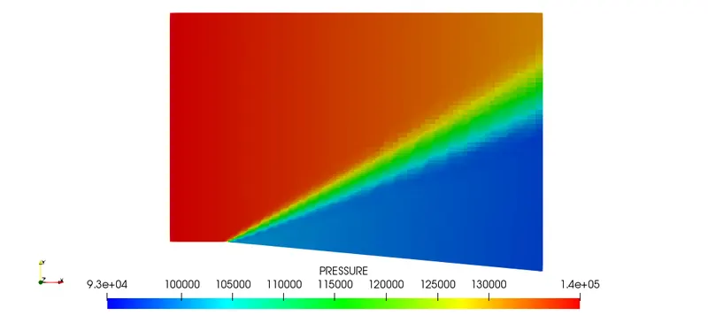
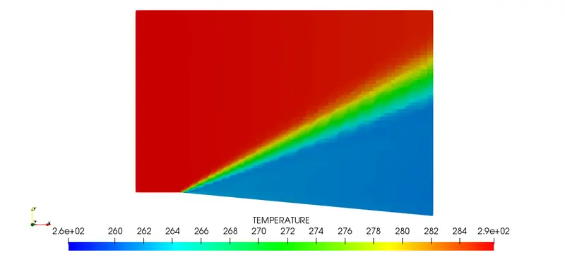
| For SGC = 0.05k | For SGC = 0.01k |
 |
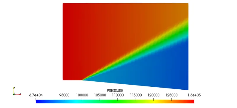 |
| Fig: Pressure contour | |
 |
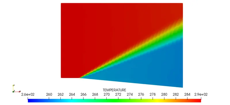 |
| Fig: Temperature contour | |
 |
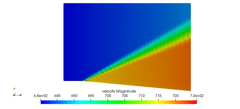 |
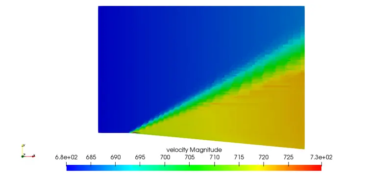
| Fig: Velocity contour | |
From all of the above contours it is seen that the contours for SGC 0.01k are smoother than contours for SGC 0.05k. It is due to the number of mesh elements which are present in more number at near flow separation. In above contours, pressure, temperature and velocity at every mesh element is shown, the lowest value is denoted in blue color and highest value is shown in red color for contours which is clear from legends. As seen in velocity contours, velocity is more than inlet velocity which is correct as per theoretical concepts. As our AMR is depend on temperature hence, very smooth temperature distribution is visible in contours.
Plots:-
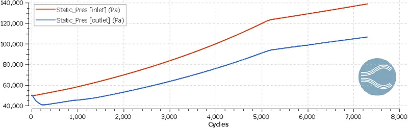 |
| Fig: Plot showing static pressure at inlet and outlet at various cycles |
|
|
| Fig: Plot showing average temperature at inlet and outlet at various cycles |
|
|
| Fig: Plot showing average velocity at inlet and outlet at various cycles |
|
|
| Fig: Plot showing mass flow rate at inlet and outlet at various cycles |
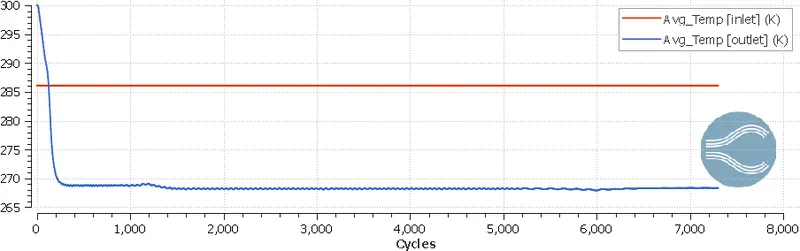
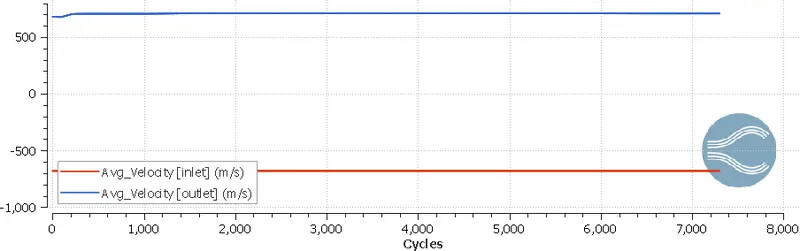
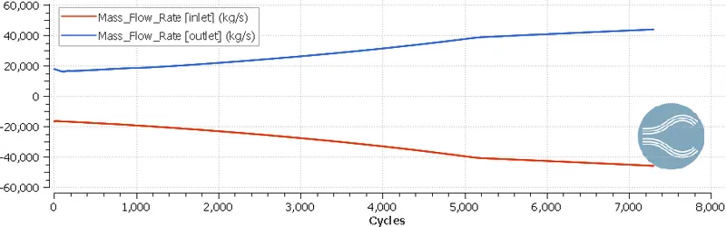
All of the above plots shows change in property with respect to number of cycles at inlet and outlet boundaries. When a plot of mass flow rate is observed, it is visible that the mass flow at inlet and outlet are of equal magnitude which indirectly shows that system is following conservation of mass rule. When static pressure plot is observed, it is clearly seen that inlet static pressure is always greater than outlet static pressure.
Note:- As the plot obtained for average temperature, average velocity, static pressure and mass flow rate are similar for both conditions (For SGC=0.05k and for SGC=0.01k) so we have attached plots of single condition only.
Temperature animation at SGC 0.05k:-
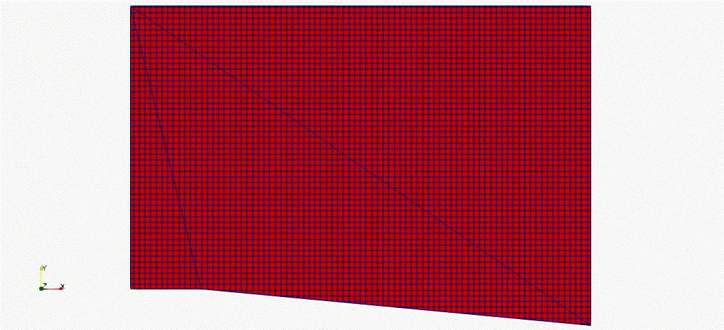
The above animation shows how meshing gets refined with respect to change in temperature. For the above animation sub grid criterion is set to 0.05k.
Temperature animation at SGC 0.01k:-
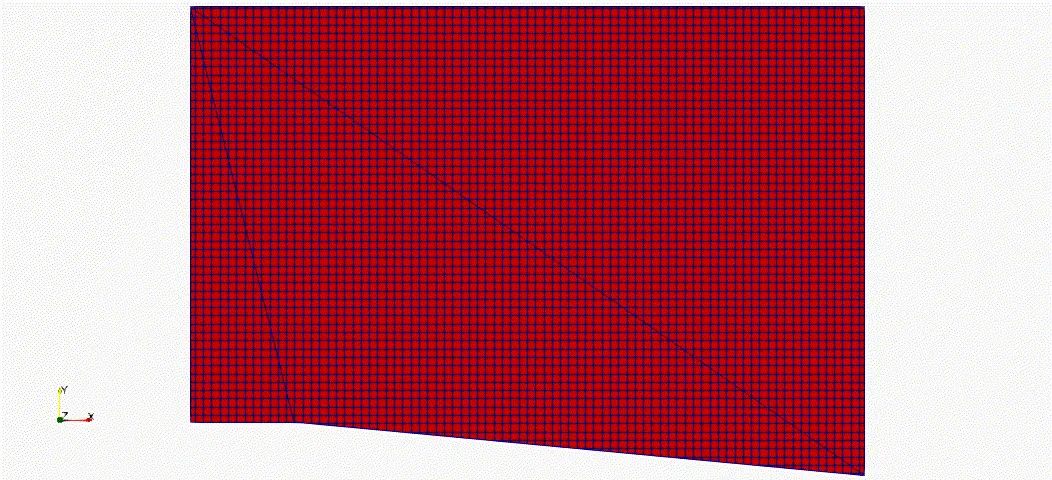
The above animation shows how meshing gets refined with respect to change in temperature. For the above animation sub grid criterion is set to 0.01k.
After comparing both animations provided above for SGC of 0.05k and SGC of 0.01k, it is observed that mesh count is quite high for 0.01k sub grid criterion, which also results in smooth contour of every properties.
Conclusion:-
- With decrease in the SGC, the mesh refinement increases and result finer mesh where change in property is in SGC limit.
- It can be seen in above example, when we provide SGC of 0.05k the mesh is refined where error in temperature is 0.05k or less than 0.05k. The error can be calculated as difference between actual temperature and resolved temperature at each cell.
- With decrease in SGC value mesh count is increased.
- Using very low value of SGC increases computational cost. The graphs at output does not vary much for low value of SGC. But while simulating flow separation problems it is good practice to use low value of SGC.
Reference:-