Conjugate heat transfer simulation of flow through pipe using Converge CFD

Aim:-> Conjugate heat transfer simulation of pipe using Converge CFD

Theory:-

As we know heat is transferred by 3 modes i.e. Conduction, convection & radiation.

1. Conduction:- is an exchange of energy by direct interaction between molecules of a substance containing temperature differences.
2. Convection:- is the transfer of internal energy into or out of an object by the physical movement of a surrounding fluid that transfers the internal energy along with its mass. Although the heat is initially transferred between the object and the fluid by conduction, the bulk transfer of energy comes from the motion of the fluid. Convection can arise spontaneously (or naturally or freely) through the creation of convection cells or can be forced by propelling the fluid across the object or by the object through the fluid.
3. Radiation:- is a transfer of thermal energy in the form of electromagnetic waves emitted by atomic and subatomic agitation at the surface of a body. Like all electromagnetic waves (light, X-rays, microwaves), thermal radiation travels at the speed of light, passing most easily through a vacuum or a nearly "transparent" gas such as oxygen or nitrogen. Liquids, "participating" gases such as carbon dioxide and water vapor, and glasses transmit only a portion of incident radiation. Most other solids are essentially opaque to radiation. The analysis of thermal radiation has a strong theoretical basis in physics, beginning with the work of Maxwell and of Planck.

Fig: Modes of Heat transfer

Conjugate heat transfer (CHT) is a type of simulation where it allows heat transfer between fluid and solid domain by exchanging thermal energy at contact surface. Here heat is exchanged at interfaces and transported by conduction process in solid and additionally by convection process within liquid. The CHT approach has an advantage over Finite element thermal analysis in that wall heat transfer coefficients and their local variations on surfaces are directly calculated within the model rather than based on simplified empirical calculations. The CHT approach therefore has benefits for those applications where heat transfer is either non-uniform or difficult to calculate empirically.

Heat transfer in solids and heat transfer in fluids are combined in the majority of applications. This is because fluids flow around solids or between solid walls and because solids are usually immersed in a fluid. Forced convection is the most common way to achieve a high heat transfer rate.

In some applications, the performances are further improved by combining convection with phase change (for example liquid water to vapor phase change). Efficiently combining heat transfer in fluids and solids is the key to designing effective coolers, heaters, or heat exchangers.

Results obtained by CHT analysis:-

1. Temperature distribution (contour).
2. Wall heat transfer coefficient
3. Heat fluxes
4. Heat transfer rate analysis
5. Realistic visualization of heat transfer
6. Identification of localized ‘hot spots’ or heat sinks in checking against specified requirements
7. Coupling CHT with FE analysis to evaluate thermally induced stresses, expansion or fatigue
8. Assessing insulation or heat shield effectiveness and optimizing of material selections

Applications of CHT analysis:-

1. HVAC
2. Heat exchanger
3. IC engines
4. Heat sink
5. Boiler
6. Turbocharger

~Pre processing:-

Geometry:

Fig: Geometry

In the above geometry of figure, the fluid enters through inlet and flows out through outlet. Fluid flows in '+ve' Z direction. The fluid is considered as air (`O_2:N_2 = 0.23:0.77`) for simulation purpose. Air with the inlet velocity of 3.467m/s which is calculated using Reynolds number 7000 entered in a domain, the inlet temperature is 300k and exit temperature also 300k. The fluid is flowing through pipe, whose material is considered as Aluminum. The heat flux of `10000W/m^2` are applied at outer (Solid) surface of pipe. Due to heat transfer, the air inside pipe gets heated as time increases.

~Problem setting:-

Simulation parameters:-

• Type of simulation: Transient state
• Gas material: Air
• Solid material: Aluminum
• Solver: Pressure based solver
• Mode: Full hydrodynamics
• Start time: 0 Second
• End time: 0.5 Seconds
• Time step: 1e-7
• Turbulence model: RNG K-epsilon
• Base grid: dx=dy=dz=0.004m
• Supercycle models: Enable
  • Supercycle point 0 = (-0.0175, 0, 0.18)

Calculation:-

Reynolds number = 7000

Characteristics length = 0.03m

But as we know, Reynold number can be calculated as-

`Re = (rhoxxVxxl)/mu`

`:. 7000 = (1.225xxVxx0.03)/(1.82*10^(-5))`

`:.V=3.467m/s`

Initial and boundary conditions:-

In above figure the boundary flagging (defining boundary) is shown, the different color denotes different boundary in geometry. There are 5 boundaries considered in simulation. Where solid region includes Aluminum as material and fluid region includes air as a material.

• Inlet: (Bound_id_3)
  • Boundary type: Inflow
  • Velocity = 3.467 m/s
  • Temperature = 300k
  • Species = Air

• Outlet: (Bound_id_4)
  • Boundary type: Outflow
  • Pressure = 101325.0 Pa
  • Velocity = Zero normal gradient
  • Temperature = 300k
  • Species = Air

• Outer solid wall:
  • Boundary type: Wall
  • Slip wall
  • Heat flux = 10000 `W/m^2`

• Solid wall:
  • Boundary type: Wall
  • Slip wall

• Interface:
  • Boundary type: Interface

Interface is a common surface (face) in two different regions. One need to define region in two different boundaries as shown in above figure.

~Post-processing:-

Case 1- Effect of Mesh refinement:

Mesh 1: 0.004m	Mesh 2: 0.00325m	Mesh 3: 0.0025m
Fig: Meshed geometry
Fig: Mesh cell count
Fig: Velocity contour
Fig: Pressure contour
Fig: Temperature contour
.
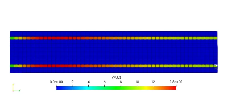
Fig: Yplus value distribution

Above contours are provided to compare the results for various meshing sizes. It is clearly visible that for fine mesh element size the distribution is smooth and more precise.

Also, in cell count line plot it is seen how number of cells are increased with decrease in mesh element size.

From the above line plots it is visible that for mesh 3 the final value is much precise than for mesh 2 and mesh 1 lines. So, it is observed that as we reduce mesh element size, we are getting much accurate results of temperature. Also, it is seen that for mesh 1 case the solution is converged more quickly than other two cases but with less precise result. If we further reduce mesh size and start simulation, t will take very high computational time but also give most accurate result. So, while performing any simulation it is much necessary to maintain mesh element size and accuracy of result.

Case 2- Effect of supercycling:

Fig: Meshed geometry

The above meshed geometry is created at baseline mesh size i.e., 0.004m cell width.

0.01	0.02	0.03
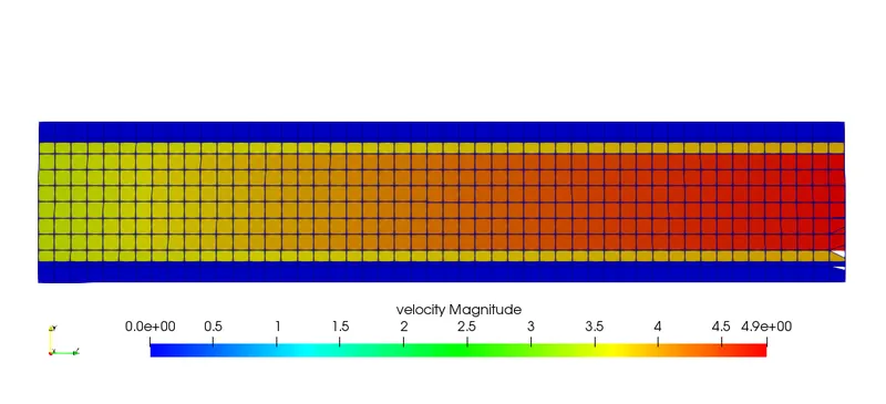Fig: Velocity contour
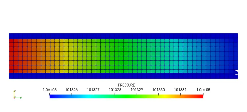
Fig: Pressure contour
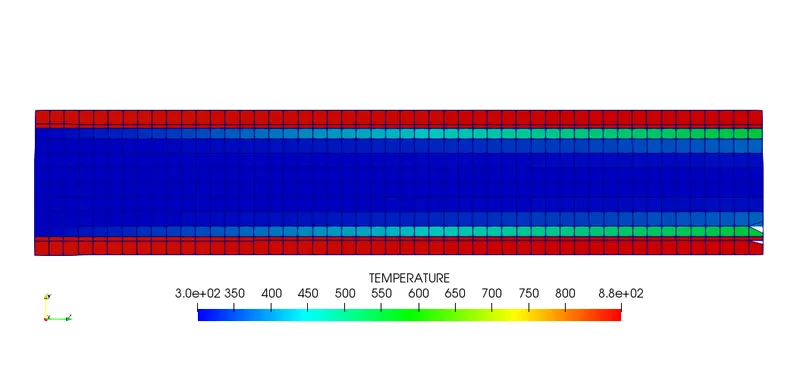Fig: Temperature contour
Fig: Yplus value distribution

While comparing all of the above contours it is seen that there is very minute difference in contours which is under tolerance value and can be neglect. So we can tell as all results are same.

It is seen from above line plots for the supercycle parameter 0.01 result converges quicker than supercycle parameter 0.02 and 0.03. Also, all the lines are converging and giving same result which means there isn't any effect of supercycling on result.

Animation of fluid flow:

The above animation is created to see how flow is propagating in fluid region. So velocity stream vectors are added to surface using glyph command and then the above animation is created.

Conclusion:- From observing all the above contours and post processed data it can be conclude that-

1. For fine meshing the results are more precise.
2. With reduction in mesh element size, the contours get smoother.
3. Supercycling parameter doesn't deviate final result.
4. For low supercycling value the result gets converged quicker than high value.