Adiabatic flame temperature calculation using Cantera
Aim:-> To calculate and observe effect of equivalence ratio, variable heat loss and variation of hydrocarbon species on adiabatic flame temperature (AFT) using python and Cantera.
Theory:-
Adiabatic flame temperature (AFT):
This temperature is defined as the temperature that is achieved by allowing fuel to react with an oxidizer. there are two types of adiabatic flame temperature depending on how the process is completed i.e. the constant volume and constant pressure. The adiabatic flame temperature is the highest temperature a system can achieve in adiabatic condition as there is no heat loss.
The constant volume adiabatic flame temperature is the temperature that results from a complete combustion process that occurs without any work, heat transfer or changes in kinetic or potential energy. Its temperature is higher than the constant pressure process because no energy is utilized to change the volume of the system.
As we know first law of thermodynamics,
`DeltaU=Q-W`
`:. U_P - U_R =(Q_(R to P)) - (W_(R to P) )`
Where,
`Q_(R to P)=` Heat transferred from reactant to product
`W_(R to P)=` Work transferred from reactant to product
`U_P" & "U_R` are the internal energy at product and reactant respectively
As work done `=W_(R to P)=int_R^P(PdV)`
`:.W_(R to P)=Pxx(V_P - V_R)`
For constant pressure,
`Delta H_p=DeltaU_p + DeltaW_p`
Here for adiabatic processes, `Delta H =0 = DeltaQ_p`
`:.H_P =H_R`
For constant volume process,
`V_P = V_R" ":. W_(RtoP)=0`
`:.Q_(v)=DeltaU`
`Q_v=Q_p - nRT =DeltaH_p - DeltanRT`
Here for adiabatic process, `Q_v = 0 =DeltaH_p -DeltanRT`
Newton Raphson method:
The Newton-Raphson method (also known as Newton's method) is a way to quickly find an approximation for the root of a real-valued function `f(x) = 0`.
It uses the idea that a continuous and differentiable function can be approximated by a straight line tangent to it. This method is mostly useful for non-linear equations.
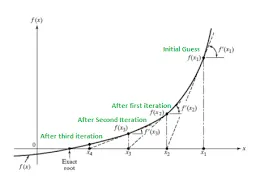
The Newton-Raphson methods require only one initial value `x_0`, which we will refer to as the initial guess for the root.
Let us consider we want to calculate roots of continuous differential function `f(x)`, then by using Newton Raphson method-
`x_1 = x_0 -(f(x_0))/(f'(x_0))`
Hence as shown in above figure, N-R process is repeated many times to obtained desired accuracy in solution.
Generelized formula for Newton Raphson method can be written as,
`x_(n+1) = x_0 -(f(x_n))/(f'(x_n))`
Combustion mechanism for methane:
The purpose of combustion in any machine is to produce heat by burning fuel. To get maximum combustion efficiency, it is important to complete burning of fuel, which is also known as complete combustion.
The reaction for the methane is as follows-
`CH_4+2(O_2+3.76N_2)<=>CO_2+2H_2O+7.52N_2`
The general reaction for any fuel is given by-
`C_xH_y+(x+y/4)(O_2+3.76N_2)<=>xCO_2+y/2H_2O+3.76xx(x+y/4)N_2`
Equivalence Ratio:
The equivalence ratio is defined as the ratio of the 'actual fuel/air ratio' to the 'stoichiometric fuel/air ratio'. Stoichiometric combustion occurs when all the oxygen is consumed in the reaction, and there is no molecular oxygen(O2) in the products.
`"Equivalence ratio"(phi)=("Actual "((fuel)/(air))" ratio")/("Stoichiometric "((fuel)/(air))" ratio")`
- If the equivalence ratio is equal to one `phi =1`, the combustion is stoichiometric.
- If `phi< 1`, the combustion is lean with excess air
- If `phi> 1`, the combustion is rich with incomplete combustion.
~Case 1:
1. Lean Mixture `(phi < 1)`
`CH_4 + 2/phi(O_2 + 3.76N_2)<=>CO_2 + 2H_2O+(2/phi-2)O_2 +7.52/phiN_2`
2. Rich Mixture `(phi >1)`
`CH_4+2/phi(O_2 +3.76N_2)<=>(4/phi -3)CO_2 + 2H_2O+(4-4/phi)CO + 7.52/phiN_2`
The enthalpy is calculated by NASA polynomials for enthalpy,
`H/(RT) = a_1 + a_2 T /2 + a_3 T^2 /3 + a_4 T^3 /4 + a_5 T^4 /5 + a_6/T`
Where, coefficients are calculated from NASA's THERM.dat file which is in CHEMKIN-II format.
Python code to calculate AFT:
'''
Program to calculate effect of equivalence ratio on AFT

Stociometric miture
CH4 + 2(O2 + 3.76N2) <-> CO2 + 2H2O + 7.52N2

LEAN MIXTURE:-
CH4 + (2/phi)*(O2 + 3.76N2) <-> CO2 + 2H2O + (7.52/phi)*N2 + (2/phi -2)*O2

RICH MIXTURE:-
CH4 + (2/phi)*(O2 + 3.76N2) <-> (4/phi -3)*CO2 + 2H2O + (7.52/phi)*N2 + (4- 4/phi)*CO

Created by: Smitesh
'''

import matplotlib.pyplot as plt
import math
import numpy as np
import cantera as ct

#By using python
R  = 8.314 #J/mol-k

# To evaluate enthalpy
def fun_1(T, coef):

	a1 = coef[0]
	a2 = coef[1]
	a3 = coef[2]
	a4 = coef[3]
	a5 = coef[4]
	a6 = coef[5]

	# NASA polynomial form for calculation of enthalpy
	# H/RT = a1 + a2 T /2 + a3 T^2 /3 + a4 T^3 /4 + a5 T^4 /5 + a6/T
	return (a1 + a2*(T/2) + a3*pow(T,2)/3 + a4*pow(T,3)/4 + a5*pow(T,4)/5 + (a6)/T)*(R*T)

CH4_coef_l = [5.14987613E+00, -1.36709788E-02, 4.91800599E-05, -4.84743026E-08, 1.66693956E-11, -1.02466476E+04]
O2_coef_l  = [3.78245636E+00, -2.99673416E-03, 9.84730201E-06, -9.68129509E-09, 3.24372837E-12, -1.06394356E+03]
N2_coef_l  = [0.03298677E+02, 0.14082404E-02, -0.03963222E-04, 0.05641515E-07, -0.02444854E-10, -0.10208999E+04]
O2_coef_h  = [3.28253784E+00, 1.48308754E-03, -7.57966669E-07, 2.09470555E-10, -2.16717794E-14, -1.08845772E+03]
N2_coef_h  = [0.02926640E+02, 0.14879768E-02, -0.05684760E-05, 0.10097038E-09, -0.06753351E-13, -0.09227977E+04]
CO2_coef_h = [3.85746029E+00, 4.41437026E-03, -2.21481404E-06, 5.23490188E-10, -4.72084164E-14, -4.87591660E+04]
CO_coef_h  = [2.71518561E+00, 2.06252743E-03, -9.98825771E-07, 2.30053008E-10, -2.03647716E-14, -1.41518724E+04]
H2O_coef_h = [3.03399249E+00, 2.17691804E-03, -1.64072518E-07, -9.70419870E-11, 1.68200992E-14, -3.00042971E+04]

n = 100
phi = np.linspace(0.1,2.0,n)

def fun_2(T,phi):

	h_CO2_p = fun_1(T,CO2_coef_h)
	h_H2O_p = fun_1(T,H2O_coef_h)
	h_CO_p  = fun_1(T,CO_coef_h)
	h_N2_p  = fun_1(T,N2_coef_h)
	h_O2_p  = fun_1(T,O2_coef_h)

	if phi > 1:
		h_product = (4/phi - 3)*h_CO2_p + (4 - 4/phi)*h_CO_p + 2*h_H2O_p + (7.52/phi)*h_N2_p
		N_p = ((4/phi -3) + 2 +(4- 4/phi) +(7.52/phi))*R*T

	else :
		h_product = h_CO2_p + (2/phi - 2)*h_O2_p + 2*h_H2O_p + (7.52/phi)*h_N2_p
		N_p = (1+ (2/phi -2) + 2 + (7.52/phi))*R*T

	T_std = 298.15
	h_CH4_r = fun_1(T_std,CH4_coef_l)
	h_N2_r = fun_1(T_std,N2_coef_l)
	h_O2_r = fun_1(T_std,O2_coef_l)

	h_reactant = h_CH4_r + (2/phi)*(h_O2_r + 3.76*h_N2_r)
	N_r = (1 + (2/phi) + (7.52/phi))*R*T_std

	return (h_product - h_reactant) - (N_p - N_r)

dT=1e-6
def fprime(T,phi):
	return (fun_2(T+dT,phi) - fun_2(T,phi))/dT

T_guess = 1500
tol = 1e-4
alpha = 0.5
temp = []

for i in phi:
	while(abs(fun_2(T_guess,i)) > tol):
		T_guess = T_guess - alpha*(fun_2(T_guess,i)/fprime(T_guess,i))
	temp.append(T_guess)

#By using cantera
gas = ct.Solution('gri30.xml')

TEMP = np.zeros(n)

for j in range(n):

	n_CH4 = 1
	n_O2  = 2/phi[j]
	n_N2  = 7.52/phi[j]
	n_t = n_CH4 + n_O2 + n_N2

	gas.TPX = 298.15, 101325, {'CH4':n_CH4/n_t, 'O2':n_O2/n_t, 'N2':n_N2/n_t}
	gas.equilibrate('UV','auto')
	TEMP[j] = gas.T

print (temp, TEMP)

#Plotting
plt.plot(phi,temp,color='red',label='Python')
plt.plot(phi,TEMP,color='blue',label='Cantera')
plt.grid('on')
plt.legend(fontsize = 12)
plt.xlabel('Equivalence ratio (phi)')
plt.ylabel('Adiabetic flame temperatur (AFT) in K')
plt.title('Equivalent ratio V/S AFT')
plt.show()
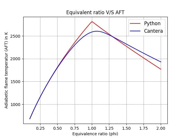
Above figure shows effect of equivalence ratio on Adiabatic flame temperature. There are two different approaches are used in above code to observe effect of equivalence ratio. At first numerical method i.e. Newton Raphson method is used and in second approach, we have used Cantera. The conditions of constant volume is considered for solving.
As the equivalence ratio increases the AFT also increases till attaining stochiometric fuel mixture i.e till equivalence ratio of 1 and then AFT decreases with increase in equivalence ratio. At equivalence ratio of 1 we get maximum AFT.
~Case 2:
As there is heat loss factor present which defines there is no adiabatic adiabatic process present for this case.
Here we have used numerical (Newton Raphson method) approach to obtain solution AFT.
Python code to calculate AFT at variable heat loss:
"""
Program to calculate effect of heat loss on AFT

Stochiometric equation
CH4 + 2(O2 + 3.76N2) <-> CO2 + 2H2O + 7.52N2

"""

import matplotlib.pyplot as plt
import math
import numpy as np

#By using python
R  = 8.314 #J/mol-k

# To evaluate enthalpy
def fun_1(T, coef):

	a1 = coef[0]
	a2 = coef[1]
	a3 = coef[2]
	a4 = coef[3]
	a5 = coef[4]
	a6 = coef[5]

	# NASA polynomial form for calculation of enthalpy
	# H/RT = a1 + a2 T /2 + a3 T^2 /3 + a4 T^3 /4 + a5 T^4 /5 + a6/T
	return (a1 + a2*(T/2) + a3*pow(T,2)/3 + a4*pow(T,3)/4 + a5*pow(T,4)/5 + (a6)/T)*(R*T)

CH4_coef_l = [5.14987613E+00, -1.36709788E-02, 4.91800599E-05, -4.84743026E-08, 1.66693956E-11, -1.02466476E+04]
CO2_coef_l = [2.35677352E+00, 8.98459677E-03, -7.12356269E-06, 2.45919022E-09, -1.43699548E-13, -4.83719697E+04]
H2O_coef_l = [4.19864056E+00, -2.03643410E-03, 6.52040211E-06, -5.48797062E-09, 1.77197817E-12, -3.02937267E+04]
O2_coef_l  = [3.78245636E+00, -2.99673416E-03, 9.84730201E-06, -9.68129509E-09, 3.24372837E-12, -1.06394356E+03]
N2_coef_l  = [0.03298677E+02, 0.14082404E-02, -0.03963222E-04, 0.05641515E-07, -0.02444854E-10, -0.10208999E+04]
N2_coef_h  = [0.02926640E+02, 0.14879768E-02, -0.05684760E-05, 0.10097038E-09, -0.06753351E-13, -0.09227977E+04]
CO2_coef_h = [3.85746029E+00, 4.41437026E-03, -2.21481404E-06, 5.23490188E-10, -4.72084164E-14, -4.87591660E+04]
H2O_coef_h = [3.03399249E+00, 2.17691804E-03, -1.64072518E-07, -9.70419870E-11, 1.68200992E-14, -3.00042971E+04]

T_std = 298.15
h_CH4_r = fun_1(T_std,CH4_coef_l)
h_O2_r  = fun_1(T_std,O2_coef_l)
h_N2_r  = fun_1(T_std,N2_coef_l)

h_reactant = h_CH4_r + 2*h_O2_r + 7.52*h_N2_r

def fun_2(T,Qs):
	h_CO2_p = fun_1(T,CO2_coef_h)
	h_H2O_p = fun_1(T,H2O_coef_h)
	h_N2_p  = fun_1(T,N2_coef_h)

	h_product = h_CO2_p + 2*h_H2O_p + 7.52*h_N2_p
	h_loss = h_reactant - (fun_1(T_std,CO2_coef_l) + 2*fun_1(T_std,H2O_coef_l) + 7.52*fun_1(T_std,N2_coef_l))

	return h_product - h_reactant + Qs*h_loss

dT = 1e-4
def fprime(T,Qs):
	return (fun_2((T+dT),Qs) - fun_2(T,Qs))/dT

T_guess = 1500
tol = 1e-4
alpha = 0.25
temp = []
Qs = np.linspace(0,1,20)

for i in Qs:
	while (abs(fun_2(T_guess,i)) > tol):
		T_guess = T_guess - alpha*(fun_2(T_guess,i)/fprime(T_guess,i))
	temp.append(T_guess)

print(temp)

plt.plot(Qs,temp,'-*',color='green')

plt.grid('on')
plt.xlabel('Heat loss factor')
plt.ylabel('Adiabetic flame temperatur (AFT) in K')
plt.title('Heat loss factor V/S AFT')
plt.show()
Output for above program:
[2325.5981295636984, 2230.019277563448, 2133.93104968237, 2037.272945639004,
1939.975612883306, 1841.9594718151097, 1743.133025847257, 1643.3907611231075,
1542.61050509334, 1440.6500619309563, 1337.3428668014722, 1232.4922858320092,
1125.864009598835, 1017.1757017514649, 906.0825919661011, 792.1568933335716,
674.857477874772, 553.4835237297542, 427.1004110876378, 294.4144366573056]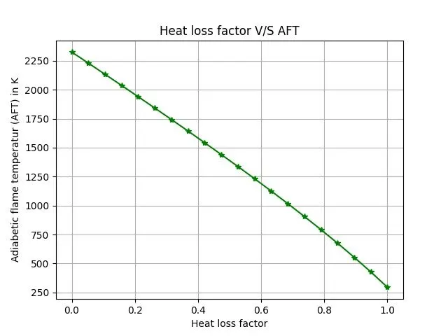
Above figure shows variation in Adiabatic flame temperature with respect to heat loss factor.
Here we have considered a constant pressure reactor with heat loss and the reactor is initially set at STP conditions i.e. 298.15K and at atm pressure.
~Case 3:
In following code, 35% of heat loss is considered.
Python code to calculate AFT with heat loss factor of 0.35:
"""
Program to calculate AFT at 0.35 heat loss factor

Stochiometric equation
CH4 + 2(O2 + 3.76N2) <-> CO2 + 2H2O + 7.52N2

"""

import matplotlib.pyplot as plt
import math

#By using python
R  = 8.314 #J/mol-k

# To evaluate enthalpy
def fun_1(T, coef):

	a1 = coef[0]
	a2 = coef[1]
	a3 = coef[2]
	a4 = coef[3]
	a5 = coef[4]
	a6 = coef[5]

	# NASA polynomial form for calculation of enthalpy
	# H/RT = a1 + a2 T /2 + a3 T^2 /3 + a4 T^3 /4 + a5 T^4 /5 + a6/T
	return (a1 + a2*(T/2) + a3*pow(T,2)/3 + a4*pow(T,3)/4 + a5*pow(T,4)/5 + (a6)/T)*(R*T)

CH4_coef_l = [5.14987613E+00, -1.36709788E-02, 4.91800599E-05, -4.84743026E-08, 1.66693956E-11, -1.02466476E+04]
CO2_coef_l = [2.35677352E+00, 8.98459677E-03, -7.12356269E-06, 2.45919022E-09, -1.43699548E-13, -4.83719697E+04]
H2O_coef_l = [4.19864056E+00, -2.03643410E-03, 6.52040211E-06, -5.48797062E-09, 1.77197817E-12, -3.02937267E+04]
O2_coef_l  = [3.78245636E+00, -2.99673416E-03, 9.84730201E-06, -9.68129509E-09, 3.24372837E-12, -1.06394356E+03]
N2_coef_l  = [0.03298677E+02, 0.14082404E-02, -0.03963222E-04, 0.05641515E-07, -0.02444854E-10, -0.10208999E+04]
N2_coef_h  = [0.02926640E+02, 0.14879768E-02, -0.05684760E-05, 0.10097038E-09, -0.06753351E-13, -0.09227977E+04]
CO2_coef_h = [3.85746029E+00, 4.41437026E-03, -2.21481404E-06, 5.23490188E-10, -4.72084164E-14, -4.87591660E+04]
H2O_coef_h = [3.03399249E+00, 2.17691804E-03, -1.64072518E-07, -9.70419870E-11, 1.68200992E-14, -3.00042971E+04]

T_std = 298.15
h_CH4_r = fun_1(T_std,CH4_coef_l)
h_O2_r  = fun_1(T_std,O2_coef_l)
h_N2_r  = fun_1(T_std,N2_coef_l)

h_reactant = h_CH4_r + 2*h_O2_r + 7.52*h_N2_r

def fun_2(T):
	h_CO2_p = fun_1(T,CO2_coef_h)
	h_H2O_p = fun_1(T,H2O_coef_h)
	h_N2_p  = fun_1(T,N2_coef_h)

	h_product = h_CO2_p + 2*h_H2O_p + 7.52*h_N2_p
	h_loss = h_reactant - (fun_1(T_std,CO2_coef_l) + 2*fun_1(T_std,H2O_coef_l) + 7.52*fun_1(T_std,N2_coef_l))

	return h_product - h_reactant + 0.35*h_loss

dT = 1e-4
def fprime(T):
	return (fun_2(T+dT) - fun_2(T))/dT

T_guess = 1500
tol = 1e-4
alpha = 0.25
ct = 0

while (abs(fun_2(T_guess)) > tol):
	T_guess = T_guess - alpha*(fun_2(T_guess))/fprime(T_guess)
	ct = ct + 1
	plt.plot(ct,T_guess,'*',color='red')

print(T_guess,ct)
plt.grid('on')
plt.xlabel('Iteration number')
plt.ylabel('Adiabetic flame temperatur (AFT) in K')
plt.title('Iteration number V/S AFT')
plt.show()
Output for above program:
1678.4119854954204
72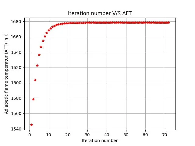
Above figure shows how AFT value is converging for 35% of heat loss. The AFT value started converging at about 20th iteration and at iteration number 72 we get final converged AFT solution of 1678.4119854954204K.
~Case 4:
For easy calculation of AFT we have used Cantera.
Python code to calculate AFT for alkane, alkene and alkyne:
#By using cantera
#Program to calculate AFT for alkane, alkene and alkyne

import matplotlib.pyplot as plt
import math
import cantera as ct

gas = ct.Solution('gri30.xml')

#For alkane
#C2H6 + 3.5(O2 + 3.76N2) <-> 2CO2 + 3H20 + 13.16N2
gas.TPX = 298.15, 101325, {'C2H6':1, 'O2':3.5, 'N2':13.16}
gas.equilibrate('HP','auto')
T_alkane = gas.T
print (T_alkane)

#For alkene
#C2H4 + 3(O2 + 3.76N2) <-> 2CO2 + 2H20 + 11.28N2
gas.TPX = 298.15, 101325, {'C2H4':1, 'O2':3, 'N2':11.28}
gas.equilibrate('HP','auto')
T_alkene = gas.T
print (T_alkene)

#For alkyne
#C2H6 + 2.5(O2 + 3.76N2) <-> 2CO2 + H20 + 9.4N2
gas.TPX = 298.15, 101325, {'C2H2':1, 'O2':2.5, 'N2':9.4}
gas.equilibrate('HP','auto')
T_alkyne = gas.T
print (T_alkyne)

Temp = [T_alkane, T_alkene, T_alkyne]

plt.figure()
plt.bar(['Ethane', 'Ethene', 'Ethyne'],Temp)
plt.ylabel('Adiabetic flame temperatur (AFT) in K')
plt.title('AFT for various hydrocarbon fuels')
plt.show()
Output for above program:
2258.73770268837
2368.6402100532237
2539.6720371204783
The above output shows adiabatic flame temperature for ethane, ethene and ethyne respectively in kelvin.
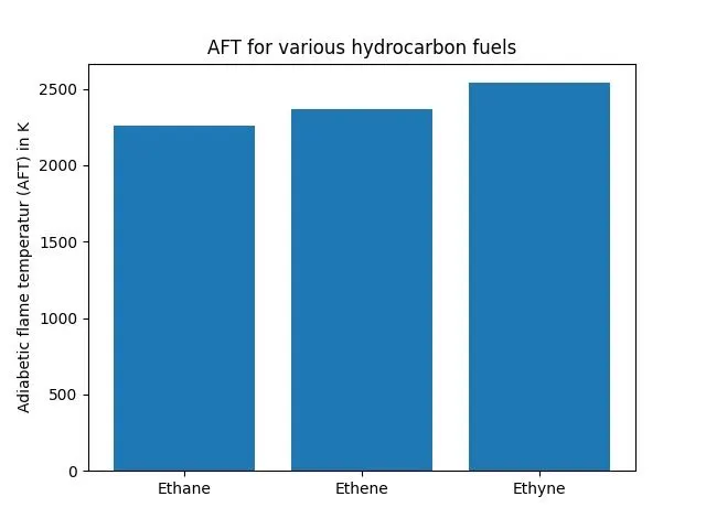
Above figure shows bar graph of hydrocarbon species v/s adiabatic flame temperature. From above graph it is seen that for same number of carbon atoms but with different number of bonds AFT varies.
~Case 5:
Python code to calculate AFT for variable carbon atoms:
#Program using cantera
#Effect of AFT for increse in carbon atom for alkane

import matplotlib.pyplot as plt
import math
import cantera as ct

gas = ct.Solution('gri30.xml')

#For C=1 (Methane)
#CH4 + 2(O2 + 3.76N2) <-> CO2 + 2H20 + 7.52N2
gas.TPX = 298.15, 101325, {'CH4':1, 'O2':2, 'N2':7.52}
gas.equilibrate('HP','auto')
T_CH4 = gas.T
print (T_CH4)

#For C=2 (Ethane)
#C2H6 + 3.5(O2 + 3.76N2) <-> 2CO2 + 3H20 + 13.16N2
gas.TPX = 298.15, 101325, {'C2H6':1, 'O2':3.5, 'N2':13.16}
gas.equilibrate('HP','auto')
T_C2H6 = gas.T
print (T_C2H6)

#For C=3 (Propane)
#C3H8 + 5(O2 + 3.76N2) <-> 3CO2 + 4H20 + 18.8N2
gas.TPX = 298.15, 101325, {'C3H8':1, 'O2':5, 'N2':18.8}
gas.equilibrate('HP','auto')
T_C3H8 = gas.T
print (T_C3H8)

Temp = [T_CH4, T_C2H6, T_C3H8]

plt.figure()
plt.bar(['Methane (CH4)', 'Ethane (C2H6)', 'Propane (C3H8)'],Temp,color='red')
plt.ylabel('Adiabetic flame temperatur (AFT) in K')
plt.title('Effect of number of carbon atoms on AFT')
plt.show()
Output for above program:
2224.6173595315677
2258.7377026884064
2265.701269069159
The above output shows adiabatic flame temperature for methane, ethane and propane respectively in kelvin.
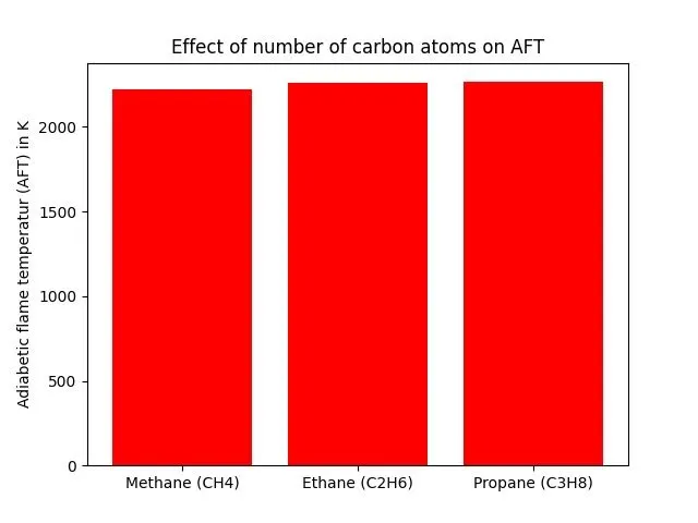
Above figure shows bar graph of various hydrocarbon species v/s adiabatic flame temperature. It seen from above graph there is no very large difference in AFT for methane, ethane and propane. But as numbers of carbon atoms increases, the temperature also increasing slightly.
Library used in python:-
- matplotlib.pyplot:- This is used to enerate plots
- math:- Includes mathematical symbols, function and arguments
- numpy:- It allows scintific computing in python
Cantera commands used:-
The gas.TPX command is used to define STP conditions at the beginning of the combustion process.
The gas.equilibrate command helps us to define which parameters we need to calculate, in this case we are computing the adiabatic flame temperature by using command gas.T.
Conclusion:- From all of the above plots and output we can conclude that-
- Adiabatic Flame Temperature obtained in case 1 using python script is less than Cantera, as there are number of small amounts of products and pollutants generated after combustion are not included in python scripting.
- The AFT increases till equivalence ratio of 1 and then decreases with increase in equivalence ratio.
- The highest AFT obtained at stochiometric mixture i.e. at `phi=1`
- With increment in heat loss value, adiabatic flame temperature decreases.
- With increase in number of bonds adiabatic flame temperature increases. For alkanes the (AFT) temperature is lower than alkene and alkyne.
- The number of carbon atoms increases in alkane results increase in AFT.