Discretization of 3D intake manifold using GEM-3D

Aim:-> To perform discretization of intake manifold with converting it in 1D circuit model from 3D model and observing effect of discretization length on result.

Theory:

Discretization is the splitting of large parts into smaller sections to improve a model's accuracy. There are two ways in which a fluid system is discretized. The first is to break the system up into several different components such as several pipes and/or flow-splits. The second is by discretizing a 'Pipe' part in to multiple sub-volumes, each performing their own calculations. When a pipe is discretized (by selecting discretization length to be shorter than the pipe length) the result will be the same as if several shorter single-volume pipes would have been used instead of one longer pipe.

Coarse discretization (larger discretization lengths) will normally result in faster simulation time, but sometimes this is at the expense of accuracy. Finer discretization may result in better accuracy and resolution, but with longer computational times. There is a limit at which decreasing the discretization length provides little or no increase in accuracy, and only adds computational time. The ideal solution is to find that limit to obtain the best accuracy with good computational time.

The discretization lengths will affect computational time in a slightly different way for each solution method. For both the explicit and implicit solution methods, computational time will be higher for smaller discretization lengths, because there will be more sub-volumes in the system that require calculation of pressure, temperature, etc. In other words, there are more solution variables. In the explicit solution method, the discretization length also affects the simulation time step. The time step is proportional to the discretization length due to the Courant condition. Smaller discretization lengths will require smaller time steps, and thus more computational time. For the implicit solution method, the time step is imposed as a constant value, and therefore simulation time is just a function of the number of sub-volumes in the system.

• Explicit solution method: an increase of computational time by a factor of ~4. The time step will decrease by a factor of 2 due to the Courant condition and there will be twice as many sub-volumes which require calculation.
• Implicit solution method: an increase of computational time by a factor of ~2. Remember that the time step in the implicit method is imposed as a constant value, so it is not affected by the discretization length. Since there are twice as many sub-volumes, there will be twice as many solution variables, resulting in an increase of computational time by a factor of ~2.

~To evaluate effect of discretization length on performance result:

~Circuit model:

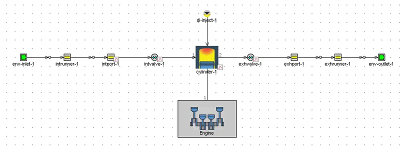
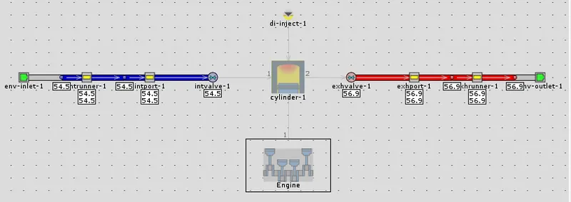
The following figure shows circuit model of single cylinder DI engine. To vary discretization length parameter called "D_length". For case 1 the length is kept as default and for case 2 it is changed to 0.1mm. The engine speed for both cases is same i.e., 3600 RPM.

~Performance result:

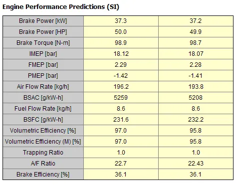
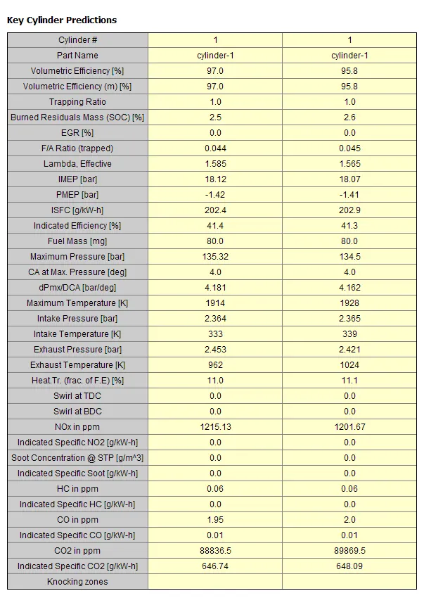
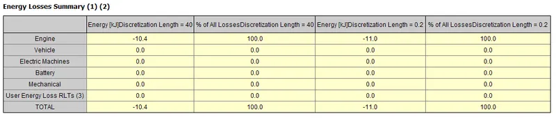
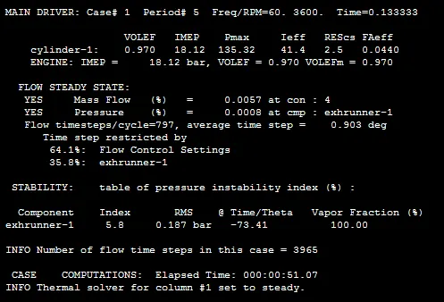
It is observed from above figures, there is very slight difference in result values for both cases i.e., for discretization length 40mm and 0.1mm.

~Computational time:

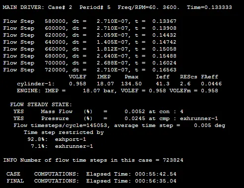Fig: For case 1	Fig: For case 2

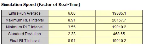
It is seen from above computational time second case took much higher time than first case.

~Mass flow contour:

Fig: For case 1

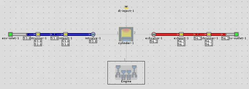Fig: For case 2

So from all the above data it is observed that one need to balance the computational time and accuracy of the result by choosing appropriate discretization length.

~Conversion of 3D model to 1D circuit model:

3D model to convert:

• Import STL file (Planum.stl) of intake manifold from example folder of GT.

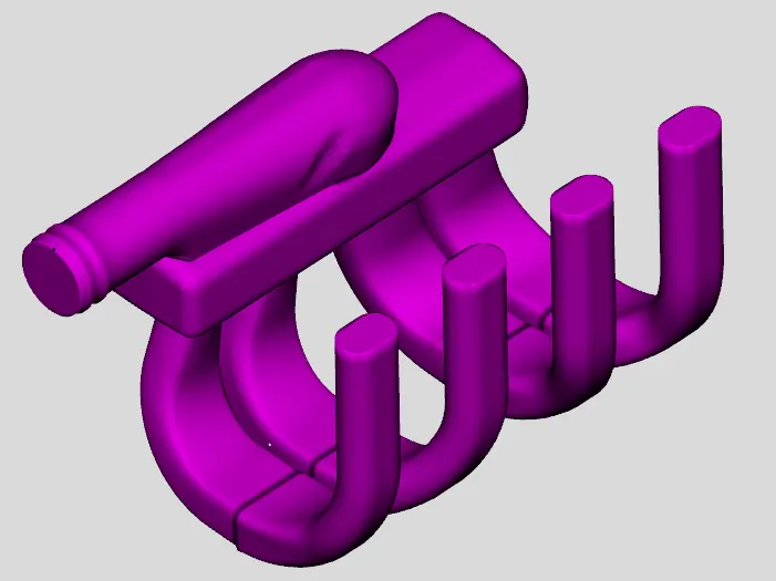
Step 1:

• Choose separate by curves command from the shape operations group in the convert tab. It will separate the surfaces on base of abrupt change in surface. A tolerance of 1 must be provided to this operation.
• As surfaces are separated which can be seen in different colors. Then end sections are separated from planum and main geometry so let us delete them to available for flow.

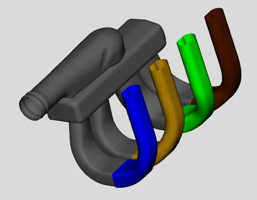
Step 2:

• Now let us separate runners from manifold. To perform this operation we need to generate cutting plane in between manifold and runners.
• Choose 3 point cutting plane command from the cutting plane group in the convert tab. Then add 3 points to generate plane on manifold appropriately. One can adjust angles and translation of cutting plane using manipulating window which is open after previewing plane.
• By clicking clip option create cutting plane and split the object in two parts. Before splitting select the object which is needed to split.

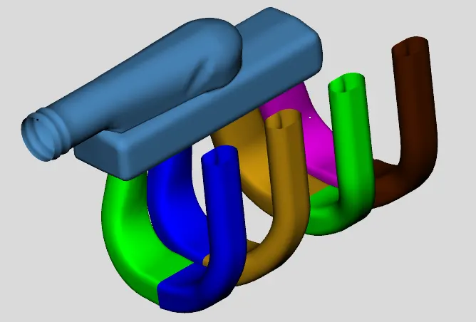
Step 3:

• Now as we have splitted geometry in multiple parts, lets convert those splitted parts into components like pipe or flow-split.
• select one runner near to manifold side and convert it into pipe with multiple bends. Before that check the flow direction, it must be from end with label 1 to label 2.
• Keep diameter of second end is same as first end.
• Then in main tab we need to set initial state object as 'init' then provide values of pressure as 1 Bar, temperature 300K and composite as a 'FluidMixture air'.
• Provide imposed wall temperature as 300K in thermal tab.
• Similarly, convert the remaining three runners to pipe and diameter of all the pipe must be similar.

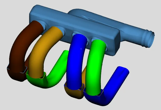
Step 4:

• Now we need to convert runner end (other part of runner which is still not converted into pipe) into pipe component. So to do that again choose any one runner and then click on 'convert shape into component' option.
• Again check direction of flow and make it correct if its opposite.
• As it is seen from geometry that both the ends of runner end are of different diameter so its needed to provide two diameters for ends. Also as there are multiple bends present pipe so choose multiple bends option.
• We have generated initial state object already so use same object here also.
• Similarly convert remaining runners into pipe.
• It is notice that there is an extra surface created by the Separate by Curves operation that we performed earlier. This surface is the vertical face of the intake runner where the diameter abruptly changed. Since this surface is not really physical, we can easily delete this surface by simply clicking on it, and pressing the delete key.

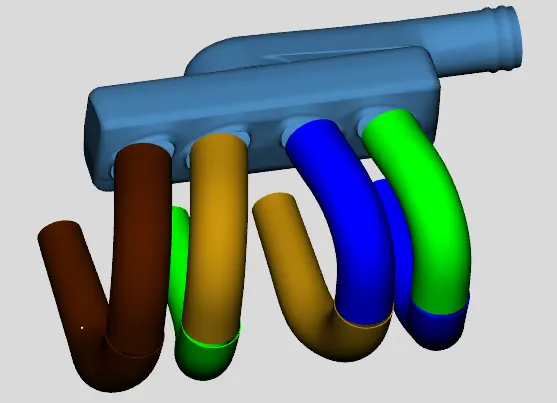
Step 5:

• In the conversion process for the runners, information regarding the curved entry from the manifold (fillets) was lost. This curved entry would represent a better flow transition than a default orifice connection, so we need to manually add an orifice connection to represent this.
• Custom orifice is added by using 'add connection' command and choose 'orificeConn' as connection type.
• Provide forward discharge coefficient as 0.95 and we need to repeat same procedure for all the remaining orifices.
• The next thing we want to do is specify the end (outlet boundary) connections, and can be done by subassembly connection.
• Then choose runner end and using command 'add connection' generate end as outlet for that choose port 2 with 'GEMSubAssExtConn' type of connection.
• Give port id as 1 for first port. Repeat this procedure for remaining ports and provide them id as 2, 3 and 4.

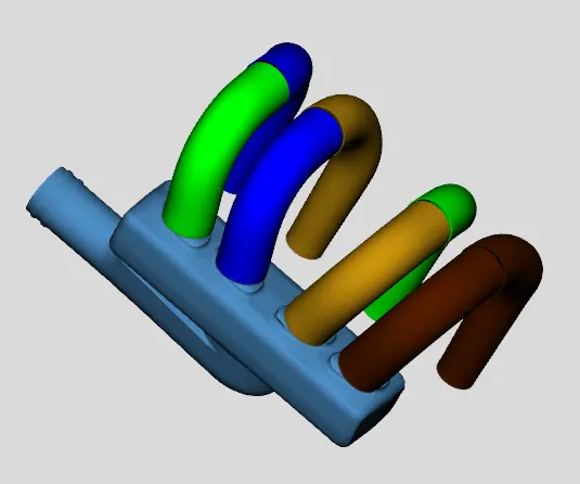
Step 6:

• Now that we have the runners converted, let's move to the other end of the manifold. The entrance appears to consist of a pipe section with a round and D-shape, then a 90 degree turn into the manifold. The straight section can be converted into 2 pipes, one representing each effective diameter.
• Let us cut it into sections so we can convert them easily into pipe. To cut section again choose cutting plane from convert tab and select 'pipe normal cutting plane'.
• Cut the manifold in three parts and convert them into pipe same as performed in previous steps.
• Again choose manifold end and using command 'add connection' generate end as inlet, for that choose port 1 with 'GEMSubAssExtConn' type of connection. Also provide port id as 5.

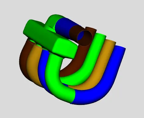
Step 7:

• The next step is to separate the manifold from the 90 degrees entrance flow-split so use 3 point cutting plane to separate it. Once the cutting plane has been created, it must be rotated slightly so that it does not cut through either the manifold or the flow-split part. Use angle and translate option to create appropriate plane.
• Once the cutting plane is in the correct orientation and location, select the mesh shape to be cut (it should display in magenta), and press the clip button in the control window.
• Now that the entrance to the manifold is separated, we can convert it into a flow component and it can be done by 'convert shape to component' command.
• Convert it into flow split object.
• Now we need to discretize large volume of manifold into small sections.
• Select 3 point cutting plane and split manifold into three sections.
• Convert all those sections into flow split component using command 'convert shape to component'.
• You will notice that during the process of converting meshes to components, we created several pipes which do not align perfectly. To remedy this, we can use the flow connection operation to join the runner sections at the top of the manifold. To do this, select 'Flow Connection > Flow Connection from the Connections group' under the tab Flow.
• To join the runners together, click on the flow connection face at the end of the first intake runner, then click on the flow connection face at the end of the second intake runner. The sections should join together.
• Similarly join the other three runners together and manifold also.
• It is seen that all four of the runners are not connected to their adjacent connections on the plenum. This is merely an artifact of the mesh-to-component conversion process. We need to add a flow connection between the plenum and intake runner pipes.
• To add a flow connection while preserving the geometry that we have displayed in GEM3D, we can add an Extruded Connection. To do this, select Extruded Connection from the Connections group in the Flow tab. All the faces which are available for adding extruded connections appear, just as with flow connections.

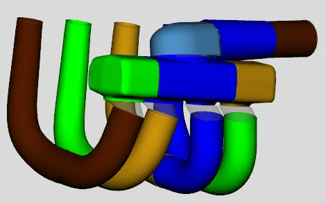
Circuit model:

• Now that the model consists entirely of flow components, we can discretize the model.
• First, save the model again using the save toolbar button or choosing Home/Save. To discretize a model, select Export GT Model from either the Home tab or the toolbar. This will open the discretization window that contains the available discretization options.
• Let's use a pipe discretization length of 40 mm and make sure the output file name is "IntMan.gtsub". Once these are correct, we need to choose an orientation for the model.
• When GEM3D discretizes the model, it will need to place each component on a 2D map in GT-ISE. It will do this based on the current graphical orientation of the model by trying to match the parts placement.
• Since the GEM3D placements are 3D and the GT-ISE map is 2D, the orientation must be carefully chosen as some orientations will result in messy model files. Rotate the model to a best possible orientation.
• Once the model is in this orientation, click the Discretize button and GEM3D will create a GT-SUITE model file (.gtsub). You will get a message saying the discretization completed successfully.
• Press the Open in GTISE button to open the newly created model file in GT-ISE. The model file map will look like the image same as model is placed in GEM3D. If the map placement is not very good, it is very easy to go back to GEM3D, rotate the model to a new orientation, and discretize the model again. Or one can easily align model in GTISE itself.

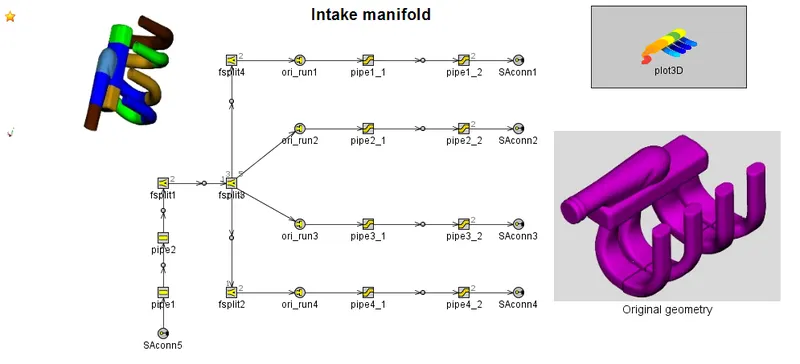
Hence by using above steps one can easily discretize 3D model and can convert into circuit model as shown in above figure.

Reference:

1. GEM3D Tutorial guide
2. GT-Suit flow theory guide.