Analysis of Cyclone Separator using discrete phase method (DPM)

Aim:-> To perform CFD analysis on cyclone separator.

Theory:-

Cyclone separator:- It is the separation devices which works on principle of inertia to remove particulate matter from flue gases. Cyclone separators is one of many air pollution control devices, known as pre-cleaners since they generally remove larger pieces of particulate matter. This prevents finer filtration methods from having to deal with large, more abrasive particles later on.

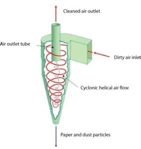Fig: Cyclone dust collector schematic diagram

Cyclone separators are generally able to remove somewhere between 50-99% of all particulate matter in flue gas. How well the cyclone separators are actually able to remove this matter depends largely on particle size. If there is a large amount of lighter particulate matter, less of these par0ticles are able to be separated out. Because of this, cyclone separators work best on flue gases that contain large amounts of big particulate matter.

All cyclone separators have an associated pressure drop. The pressure drop can be thought of as the amount of energy required to move the gas through the separator, alternatively, it can be thought of as the amount of resistance the cyclone separator adds to the system flow. The pressure drop is a product of the gas flow rate, gas density and cyclone geometry.

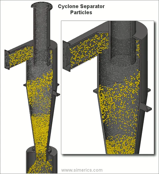Gas containing entrained particles (dirty air) enters at high velocity through the tangential inlet at the top of the cyclone. The gas flows into the cyclone body/barrel at a tangent and begins to flow in a circular downward spiral towards the lower reject port; this downward flowing spiral is referred to as a spiral vortex. Particles with more inertia will impact with the side of the cyclone whilst particles with lower inertia will remain within the gas stream. The cone diameter gradually decreases which causes the gas velocity to increase. The outer vortex creates an additional inner vortex closer to the center of the separator body and this inner vortex flows spirally upwards towards the accept port.

Particles with greater inertia will be less affected by the vortex and will continue travelling in a straight line. This straight-line trajectory causes the high inertia particles to move out of the gas stream and impact with the cyclone separator body. These particles then fall to the base of the cyclone separator and out of the reject port. In this way, entrained particles of a certain size can be separated from the gas stream.

Empirical efficiency models:-

1. Iozia and Leith model:

Iozia and Leith model is modified version of Barth model. This model is developed based upon force balance. The model assumes that a particle carried by the vortex endures the influence of two forces i.e. centrifugal force and flow resistance.

Collection efficiency of a particles with diameter `d_("pi")` can be calculated as-

`eta_i=1/(1+(d_(pc)/d_("pi"))^beta)`

Where,

`beta="Expression for slope parameter"`

`beta=0.62-0.87ln(d_(pc)/100)+5.21ln((ab)/D^2)+1.05ln((ab)/D)^2`

`d_(pc)="50% cut size"`

`d_(pc)=[(9muQ)/(pirho_pz_cv_(tmax)^2)]^0.5`

2. Li and Wang model:

Li and Wang (1989) model includes particle bounce or re-entrainment and turbulent diffusion at cyclone wall. A two dimensional analytical expression of particle distribution in cyclone is obtained.

This model based on following assumption-

-> The radial particle velocity and the radial concentration profile are not constant for uncollected particles within the cyclone.

-> Boundary conditions with the consideration of turbulent diffusion coefficient and particle bounce re-entrainment on the cyclone wall are:

`c=c_0" at "theta=0`

`D_r(delc)/(delr)=(1-alpha)omegac" at "r=D/2`

-> The tangential velocity is related to the radius of cyclone by:

`uR^n = "constant"`

The collection efficiency can be formulate as-

`eta_i=1-exp{-lambdatheta_1}`

where,

`theta_1=2pi(S+L)/a`

`lambda=((1-alpha)komega_w)/(D_rr_w^n)`

3. Koch and Licht model:

Koch and Licht collection theory recognized the inherently turbulent nature of cyclones and the distribution of gas residence times within the cyclone. Koch and Licht described particle motion in the entry and collection regions with the additional following assumptions:

• The tangential velocity of a particle is equal to the tangential velocity of the gas flow, i.e. there is no slip in the tangential direction between the particle and the gas.
• The tangential velocity is related to the radius of cyclone by:

`uR^n = "constant"`

The efficiency can be calculated as-

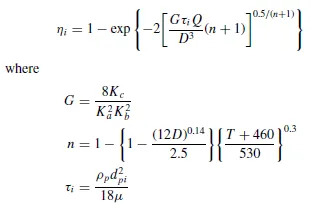
Here G is factor related to configuration of cyclone and n related to vortex.

4. Lapple model:

Lapple model was developed based on force balance without considering the flow resistance. Lapple assumed that a particle entering the cyclone is evenly distributed across the inlet opening. The particle that travels from inlet half width to the wall in the cyclone is collected with 50% efficiency.

The semi empirical relationship developed by Lapple to calculate a 50% cut diameter, dpc, is

`d_(pc)=[(9mub)/(2piN_ev_i(rho_p-rho_g))]^0.5`

Where,

`N_e = "Number of revolution"`

`N_e=1/a[(H+h)/2]`

And efficiency can be given as-

`eta_i=1/(1+(d_(pc)/d_("pi"))^2)`

Pre processing:-

It includes geometry preperation and mesh generation.

Geometry:

Fig: Geometry

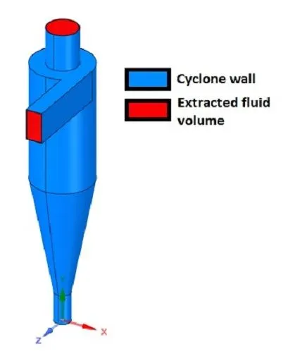
Above figure shows geometry of cyclone separator.

The 3D model of cyclone separator provided by course instructor in form of STEP file is imported in ANSYS space-claim. Then by using edge selector from volume extraction option choose inlet and outlet edges carefully to extract volume. Then extract volume by clicking on correct option. Hence we got our extracted volume. Then hide the cyclone separator body and suppressed it for physics also.

In above figure red color shows extracted volume and blue color shows cyclone separator body.

Material:

The fluid is considered as air here and the dirt particals are concider as anthracites.

Meshing:

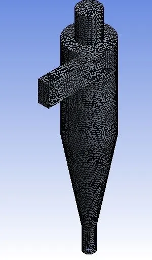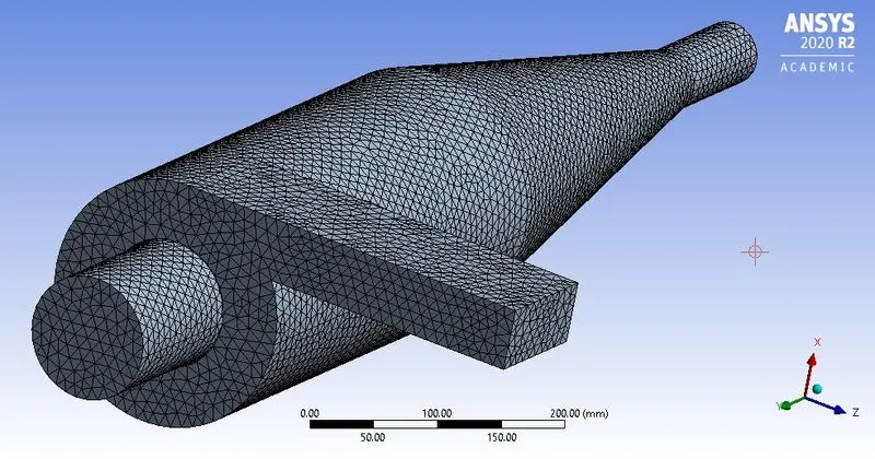Fig: Meshed geometry

Above figure shows meshed geometry.

• Mesh element size = 10mm
• Number of nodes = 34329
• Number of elements = 180377

Due to computational power limitations, we have taken mesh size of 10mm. Further refinement in mesh size is possible on high end systems.

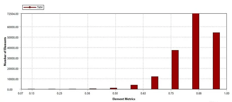
Above figure shows mesh quality matrix. As maximum number of elements are coming in between 0.5 to 1 element matrix, hence the overall quality of mesh is considered as good meshing to perform further simulation.

Solving and boundary conditions:

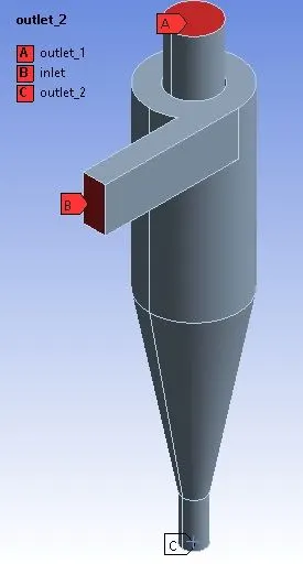Fig: Boundary conditions

After meshing select inlets and outlets using face selector and named them using named selection tool as shown in above figure.

Solver steps-

• Enable gravity in '-ve' Y direction and put value of 9.81m/s^2
• Select steady state pressure based solver
• Then select `k-epsilon` turbulent model
• Enable RNG and swirl dominated options also
• Then enable discrete phase modelling to track particle flow
• Then create injection with anthracite material and select injection type surface
• Then choose inlet face from reference surfaces
• As per conditions and case, change the velocity of anthracites and diameter of anthracite particles.

In fluent solver apply following boundary conditions-

• Inlet and wall:- Reflect
• Outlet(Top):- Escape
• Outlet(Bottom/dustbin) - Trap

Here,

1. Reflect defines particles should rebound (reflect) from given surface
2. Trap defines trajectory calculation to be stopped after touching surface
3. Escape defines calculation stops as soon as particle escape from boundary

Then vary the inlet velocity from 1m/s to 5m/s as per required cases.

And then use standard initialization where take reference values from inlet.

Post processing:-

Separation efficiency: It can be defined as ratio of number of particles within given size limit collected at drip to number of particles entered in separator.

So it can be formulate as-

`"Separation efficiency"="Number of particles trapped"/"Number of particles tracked"`

~Case 1:- With variable size

~Case 1.1:

Anthracite size 1`mum`

Velocity = 3m/s

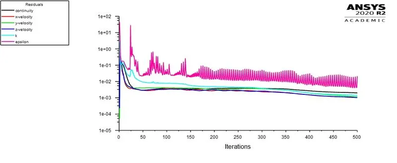
Fig: Residual plot

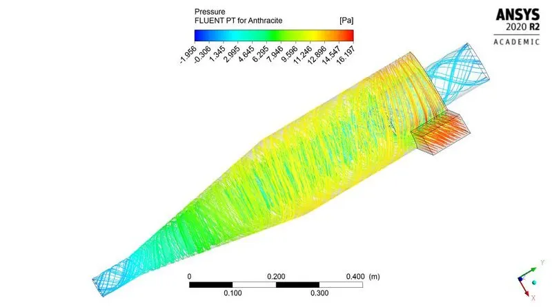
Fig: Pressure contour

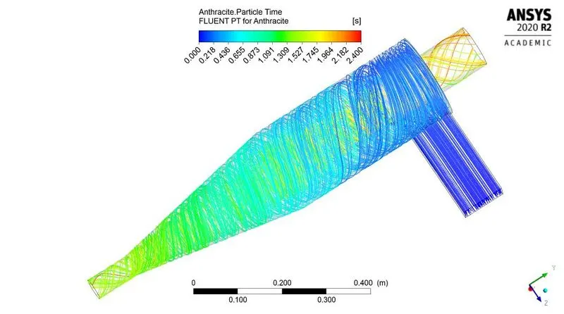
Fig: Time contour

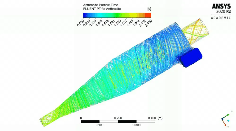
Fig: Time animation for anthracite

~Case 1.2:

Anthracite size 2`mum`

Velocity = 3m/s

Fig: Residual plot

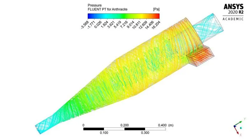
Fig: Pressure contour

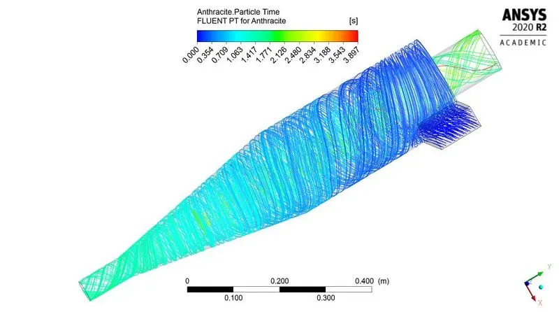
Fig: Time contour

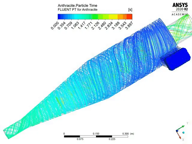
Fig: Time animation for anthracite

~Case 1.3:

Anthracite size 3`mum`

Velocity = 3m/s

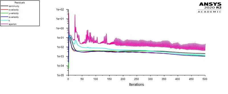
Fig: Residual plot

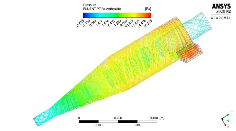
Fig: Pressure contour

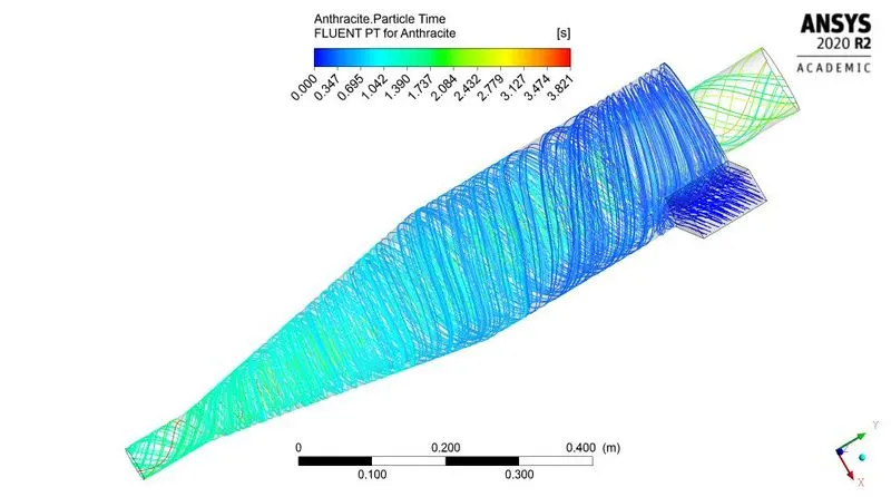
Fig: Time contour

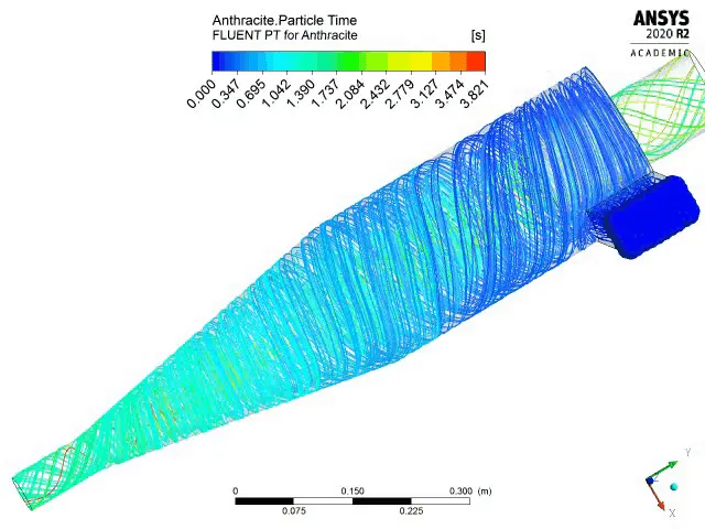
Fig: Time animation for anthracite

~Case 1.4:

Anthracite size 4`mum`

Velocity = 3m/s

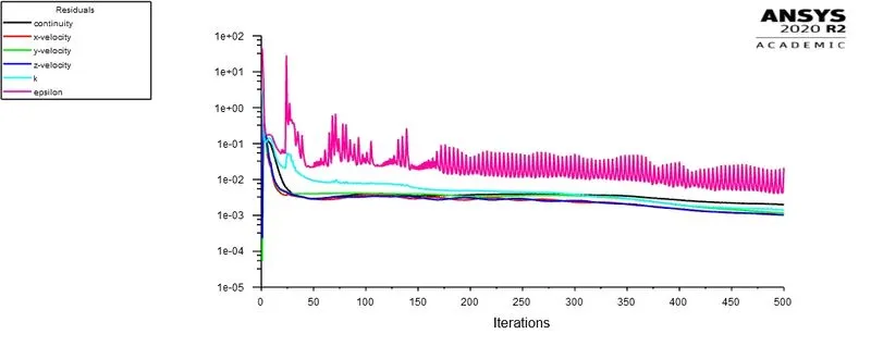
Fig: Residual plot

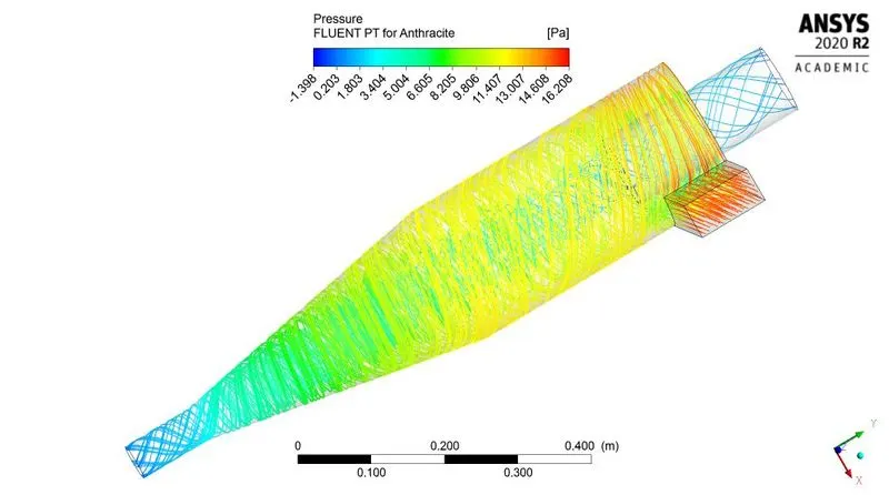
Fig: Pressure contour

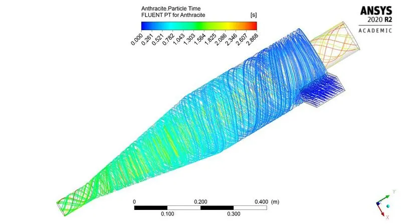
Fig: Time contour

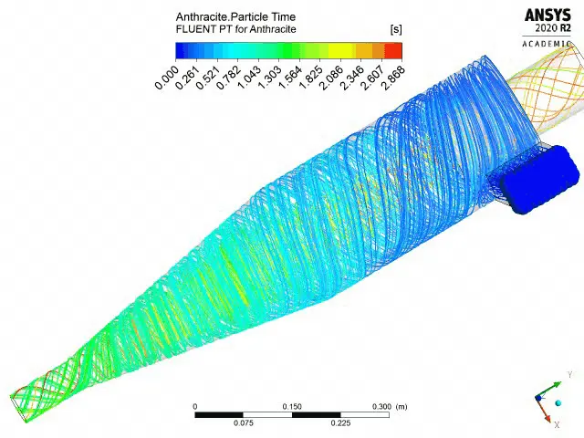
Fig: Time animation for anthracite

Anthracite particle size (`mum`)	Min pressure (Pa)	Max pressure (Pa)	Pressure difference (Pa)	Time for last particle to trapped/escaped (Second)
1	-1.956	16.197	18.153	2.4
2	-3.568	16.204	19.772	3.897
3	-3.555	16.215	19.77	3.821
4	-1.398	16.208	17.606	2.868
Table: Summery for variable anthracite size

Anthracite particle size (`mum`)	Total particles tracked	particles trapped	particles escaped	particles incomplete	Effeciency (%)
1	120	65	21	34	54.1667
2	120	93	27	-	77.5
3	120	99	21	-	82.5
4	120	106	14	-	88.3334
Table: particle data for variable anthracite size

~Case 2:- With variable velocity

~Case 2.1:

Anthracite size 5`mum`

Velocity = 1m/s

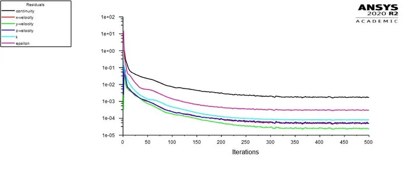
Fig: Residual plot

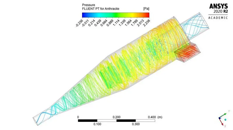
Fig: Pressure contour

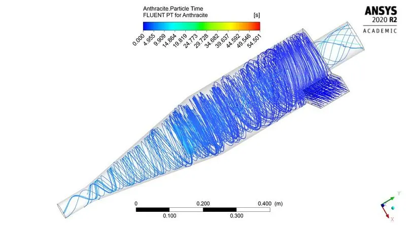
Fig: Time contour

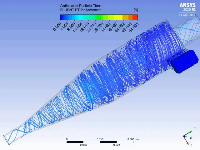
Fig: Time animation for anthracite

~Case 2.2:

Anthracite size 5`mum`

Velocity = 2m/s

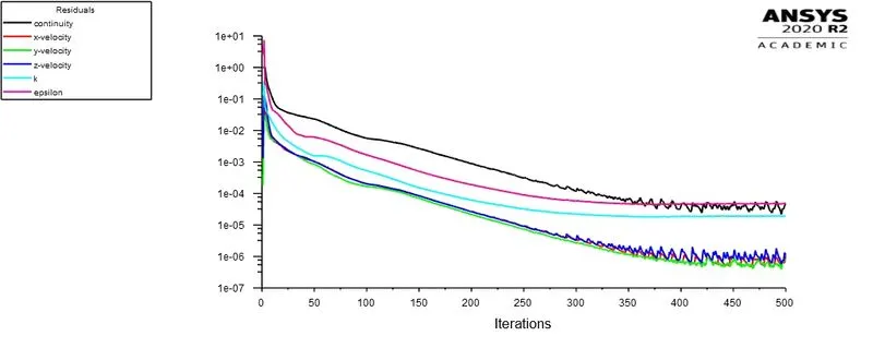
Fig: Residual plot

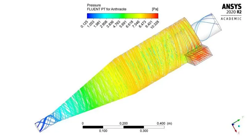
Fig: Pressure contour

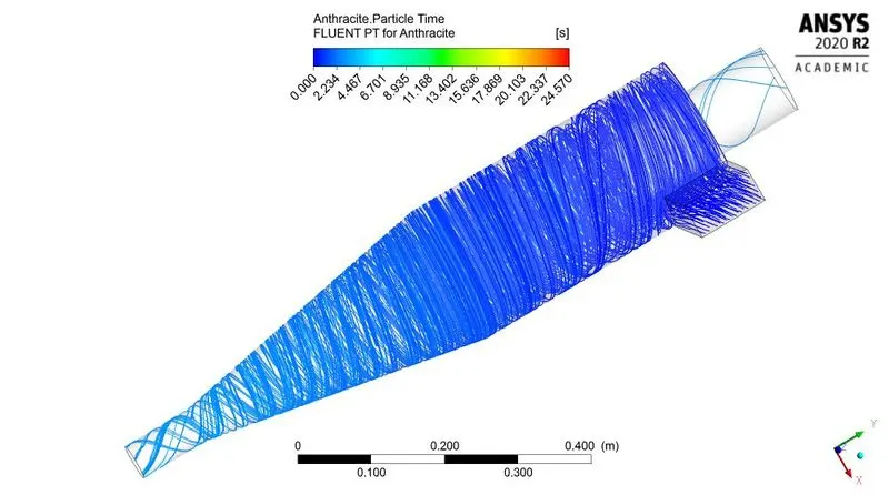
Fig: Time contour

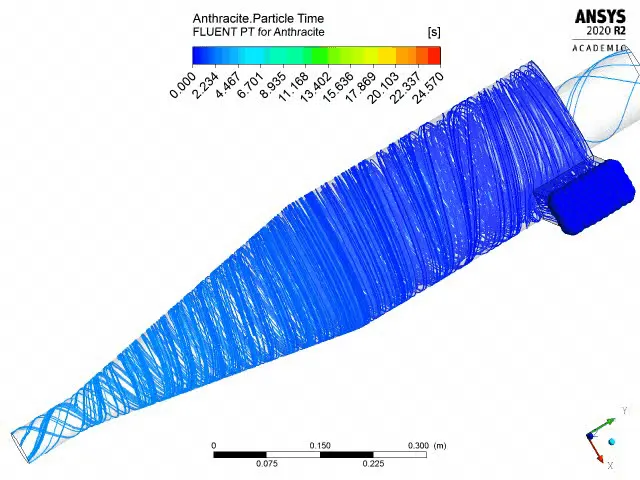
Fig: Time animation for anthracite

~Case 2.3:

Anthracite size 5`mum`

Velocity = 3m/s

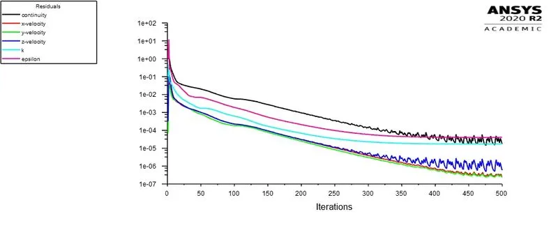
Fig: Residual plot

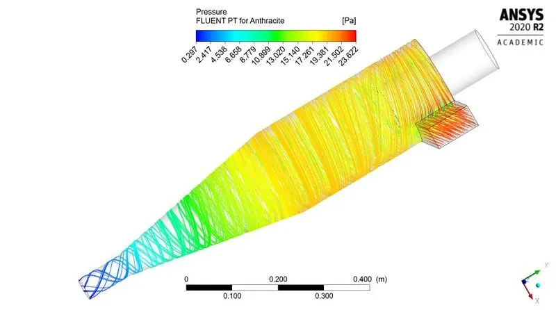
Fig: Pressure contour

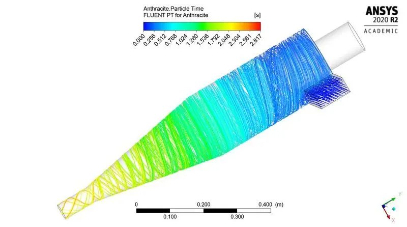
Fig: Time contour

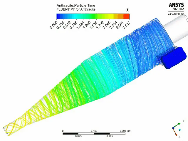
Fig: Time animation for anthracite

~Case 2.4:

Anthracite size 5`mum`

Velocity = 4m/s

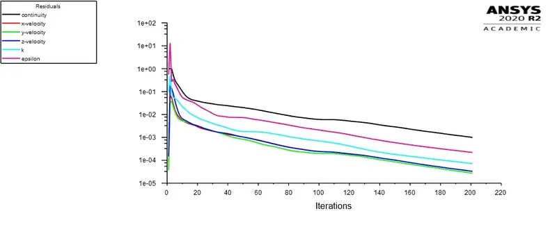
Fig: Residual plot

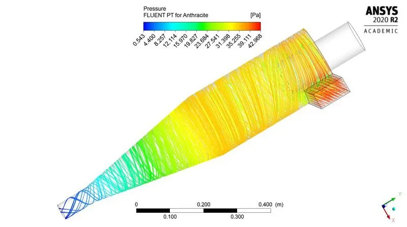
Fig: Pressure contour

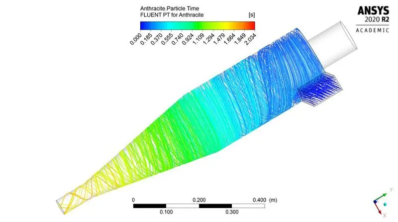
Fig: Time contour

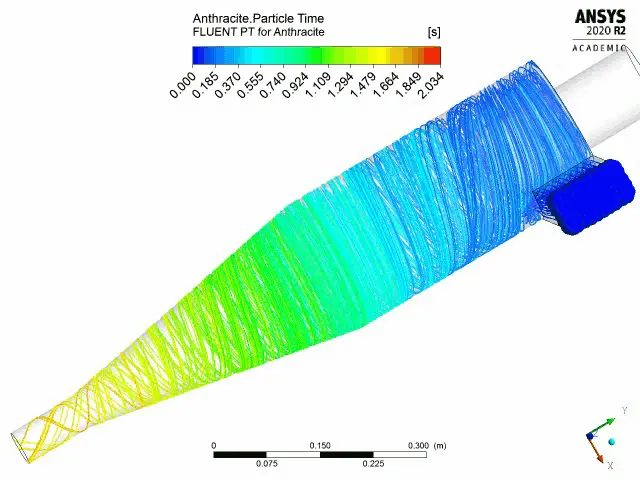
Fig: Time animation for anthracite

~Case 2.5:

Anthracite size 5`mum`

Velocity = 5m/s

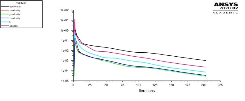
Fig: Residual plot

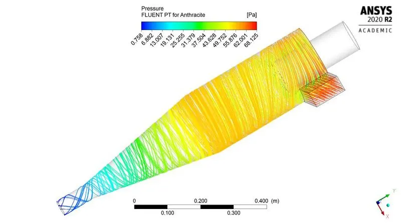
Fig: Pressure contour

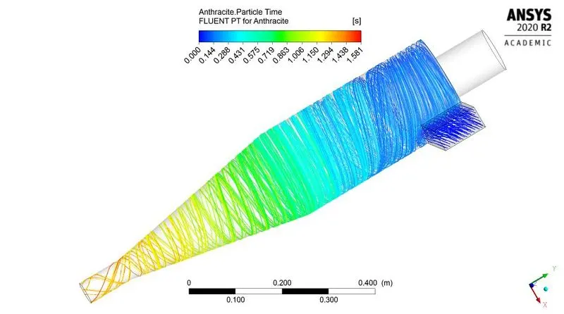
Fig: Time contour

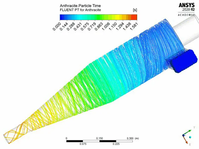
Fig: Time animation for anthracite

Anthracite particle velocity (m/s)	Min pressure (Pa)	Max pressure (Pa)	Pressure difference (Pa)	Time for last particle to trapped/escaped (Second)
1	-0.236	2.238	2.474	54.501
2	0.125	10.328	10.203	24.57
3	0.297	23.622	23.325	2.817
4	0.543	42.968	42.425	2.034
5	0.758	68.125	67.367	1.581
Table: Summery for variable anthracite size

Anthracite particle velocity (m/s)	Total particles tracked	particles trapped	particles escaped	particles incomplete	Effeciency (%)
1	120	5	10	105	4.1667
2	120	42	5	73	35
3	120	120	-	-	100
4	120	120	-	-	100
5	120	120	-	-	100
Table: particle data for variable anthracite size

For all the above plots showing residual v/s iteration we can see that the same shape is repeating which confirms that the solution is converged.

The above simulation can be improved by reducing mesh element size and by using structural cut cell meshing method, but it will take large computational memory and computational time also. Due to academic license and system restrictions we have consider above mesh settings. And we obtain results as written above.

Conclusion:-

By observing above post processed data, result and tables we can conclude that-

1. The separation efficiency is increasing with increase in anthracite particle size (particle diameter). It happens due to large inertia.
2. The separation efficiency also increases with increase in inlet velocity of particle.
3. The time required to capture last trapped particle is reduces with increase in inlet velocity.
4. With increase in velocity, pressure difefrence also increases.
5. Velocity has more effect on pressure difference, for same velocity pressure difference varies slightly.
6. By using more refined mesh, the result may vary and those results are more accurate than above obtained results.

Reference:-

A CFD study on the prediction of cyclone collection efficiency

Numerical study of gas-solid flow in cyclone separator

Cyclone separator and its working