Combustion simulation of methane injected to analyze the mass fraction of pollutants using ANSYS Fluent

Aim:-> Combustion simulation on combustor model using ANSYS fluent and to analyze effects of adding water in fuel on pollutants (NOx & Soot) generation.

Theory:-

Combustion:

Combustion or burning is a high temperature exothermic chemical reaction between a fuel (hydrocarbons) and an oxidant (air) accompanied by the release of energy in form of heat, light and unburnt gases.

In order to solve the complex equations from chemical kinetics and to yield information about the reaction mechanism proper physical modeling has to be done. In this project, the combustion process is simulated with the help of CFD software ANSYS fluent. In case of incomplete combustion, various pollutants are formed, such as carbon dioxide, carbon monoxide, nitric oxide, etc.

Combustion manifests itself as a wide domain during the design, analysis, and performance characteristics stage by being an integral part of various engineering applications like internal combustion engines, aircraft engines, rocket engines, furnaces, and power station combustors.

In ANSYS FLUENT we can use following methods for combustion simulation.

1. Based on mixing

• Non-premixed combustion
• Premixed combustion
• Partially premixed combustion

2. Based on phase

• Fluid phase (Volumetric reactions)
• Wall (surface reactions)
• Particles (surface reaction)
• Porous region (After Treatment system)

Chemical reactions:

The combustion reaction used here is

`CH_4+a_r(O_2+3.76N_2)→aCO_2+bH_2O+cN_2`

Here,

`CH_4=1` mole

Then after solving the stoichiometric equation we get,

Air i.e. `a_r(O_2+3.76N_2)= 2 O_2 + 7.52 N_2`

As we know,

Atomic weight of oxygen =16

Atomic weight of nitrogen =14

`"Mass fraction" ="Mass of molecule"/"Mass of air"`

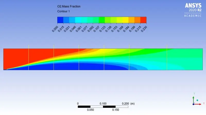
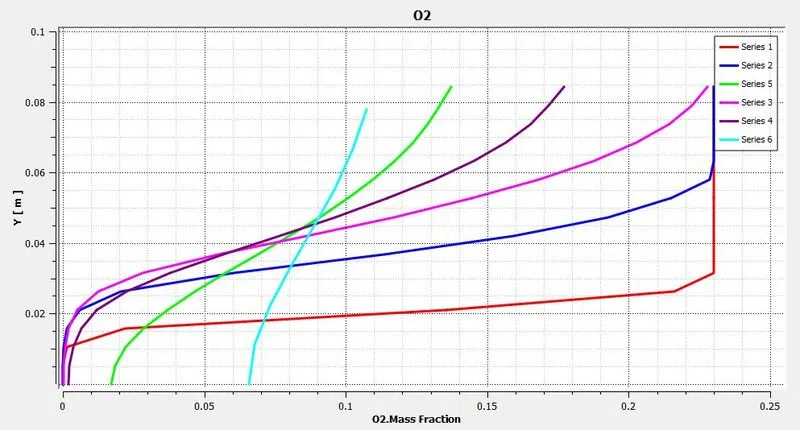
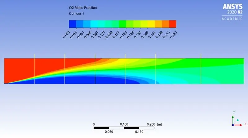
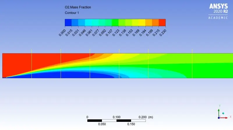
`:."Mass fraction of oxygen"=32/137.8=0.23`

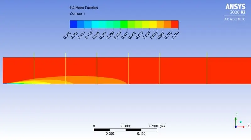
`:."Mass fraction of nitrogen"=105.8/137.8=0.77`

The following simulation is performed in two parts.

In first part the fuel methane is provided simply and the plots are obtained.

In second part of simulation the Methane fuel is added with different amount of water molecules (5% to 30% by mole) to observe NOx and soot formation.

For simplicity we have done simulation using parametric study approach. Where `CH_4" & "H_2O` considered as input parameters.

Pre-processing:

Model:-

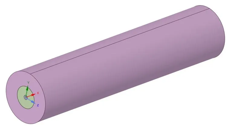
Fig: 3D Model of combustor

Above figure shows 3D model of combustor. It has small inlet for fuel in center.

Above model is very large to work on hence, instead of doing simulation on 3D model, we can simulate in 2D by created 2D geometry. As the above body is symmetric about X axis (Circular cross section) so we can use axisymmetric command to obtain similar results as 3D model in less cost and time on 2D geometry.

Steps involved in geometry preparation:

• At first open Space-claim
• Then import 3D model of combustor which is available in step format
• Then create mid plane parallel to XY plane at Z=0
• Then split the body in half by using appropriate command in "prepare" tab
• Similarly, again create plane parallel to XZ plane at Y=0
• Again, split body in half (so we will get now quarter part of original model)
• Copy the surface in XY plane
• Paste the 2D surface in new file so we get 2D surface geometry
• Now use option share topology to avoid problems in meshing
• And finally export the 2D prepared geometry in ANSYS meshing for further operations

Geometry:-

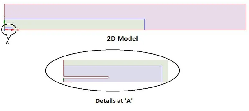
Fig: 2D axisymmetric geometry

The above picture shows 2D axisymmetric geometry of model. The geometry is axisymmetric along X axis. The detailed view (enlarge view) of geometry near fuel inlet is shown in "Details at A". From small inlet fuel is injected inside combustion chamber.

NOTE:- Remember that in ANSYS geometry should be drawn on XY plane and the axis along which geometry is axisymmetric should be X-axis only

Meshing:-

Fig: Meshed geometry	Fig: Mesh quality near Fuel inlet

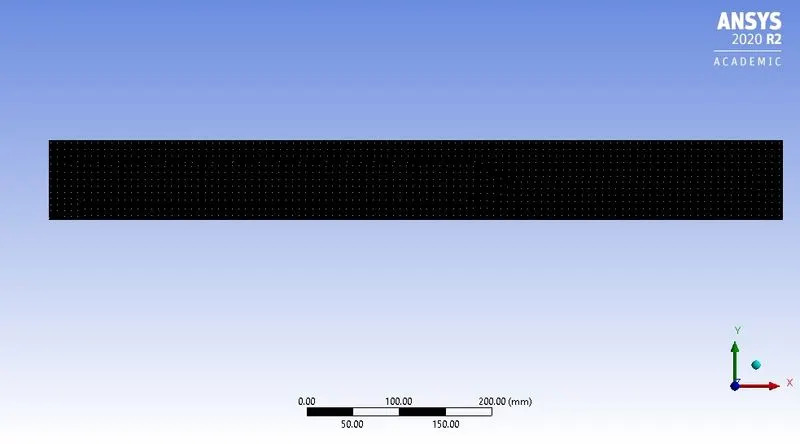
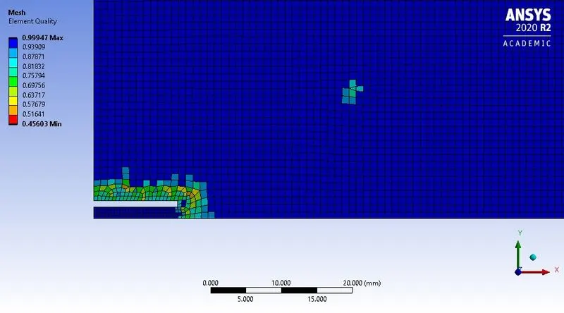
Above figures shows meshed geometry. Also in above figure most of mesh are in blue color which denotes that best quality mesh. The mesh statistics are given below-

Mesh statistics:

• Mesh element size = 1mm
• Number of nodes = 68729
• Number of elements = 67839

As "Capture proximity" option is enabled and we have provided value 4, hence the mesh is finer near fuel inlet side.

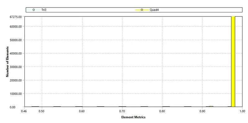
Above figure shows mesh quality matrix.

As maximum number of elements are coming in between 0.9 to 1 element matrix range, hence the overall quality of mesh is considered as good meshing to perform further simulation.

Material:-

• Fuel:- Methane `(CH_4)`

Solving and Boundary conditions:

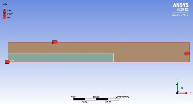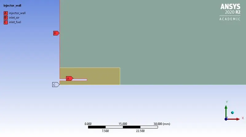The above figure label denotes boundaries for geometry.

Boundary conditions:

For fuel-

• Fuel inlet velocity = 80m/s
• Inlet temperature of fuel = 300k
• Species mass fraction for `CH_4=1;` for case 1
• Species mass fraction for `H_2O=0;` for case 1
• Species mass fraction for `CH_4` variable from 0.95 to 0.7 for case 2
• Species mass fraction for `H_2O` variable from 0.05 to 0.3 for case 2

For air-

• Air inlet velocity = 0.5m/s
• Inlet temperature of air = 300k
• Species mass fraction for `O_2=0.23`

Case setup:

1. Solver: Steady

2. Type: Pressure based

3. Axisymmetric: On

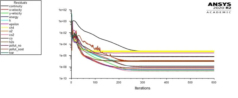
4. Turbulence model: `k-epsilon` model with Standard wall function

5. Energy model: On

6. Species model: On

• Choose species transport equation
• Enable volumetric reaction
• Enable "Inlet diffusion" and "Diffusion energy source" options
• Mixture material: Methane-air-2step
• Turbulence chemistry interaction: Eddy dissipation

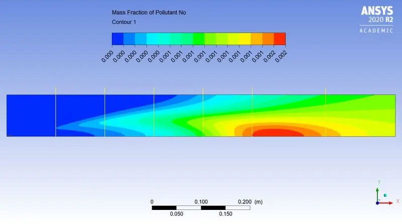
7. `NO_X` model: On

• Enable `NO_X` model with "Thermal NOx" and "Prompt NOx" options

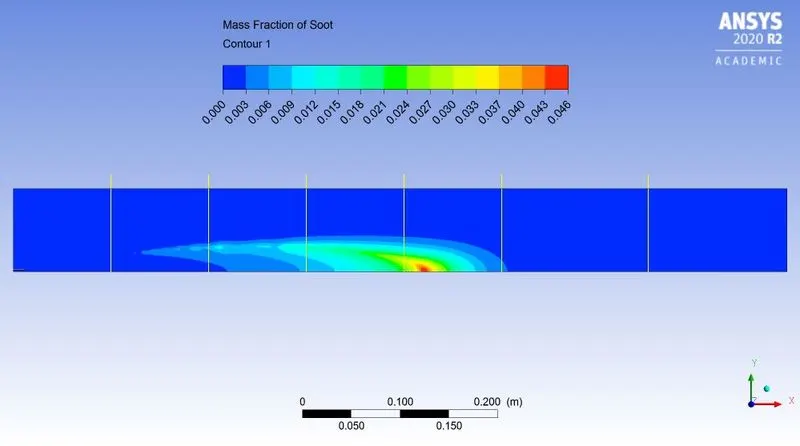
8. Soot model: On

• Use one step Soot model

9. Initialization: Standard initialization

Post-processing:

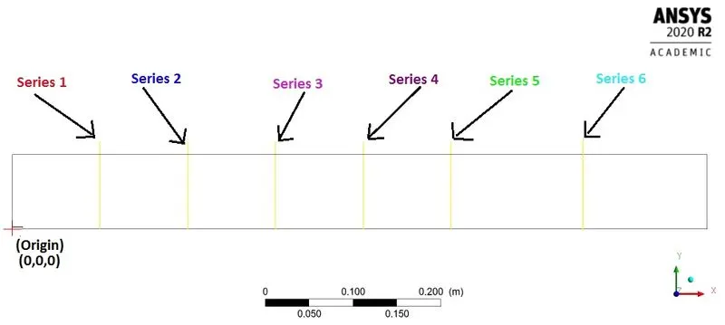
Fig: Line definitions for mass fraction

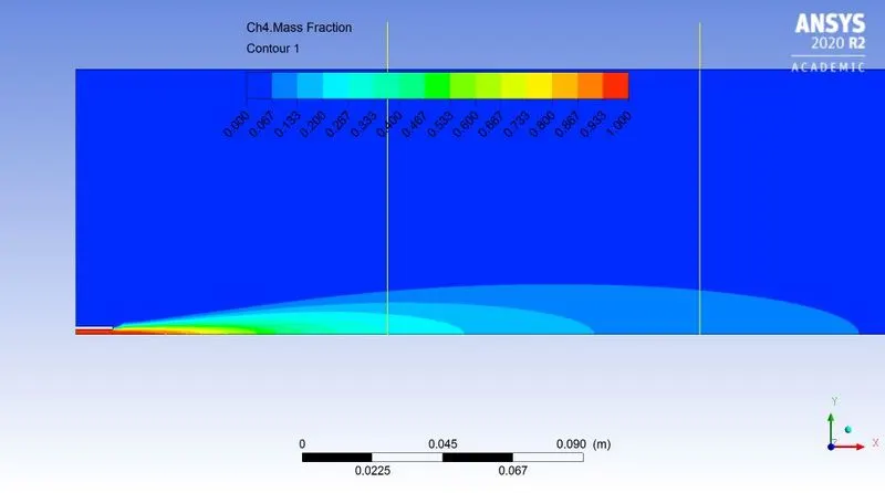
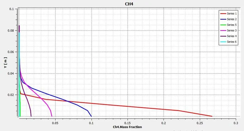
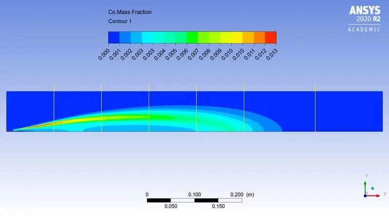
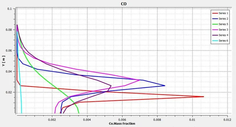
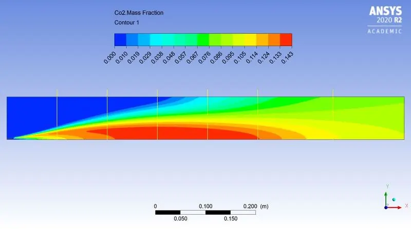
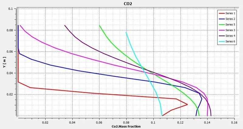
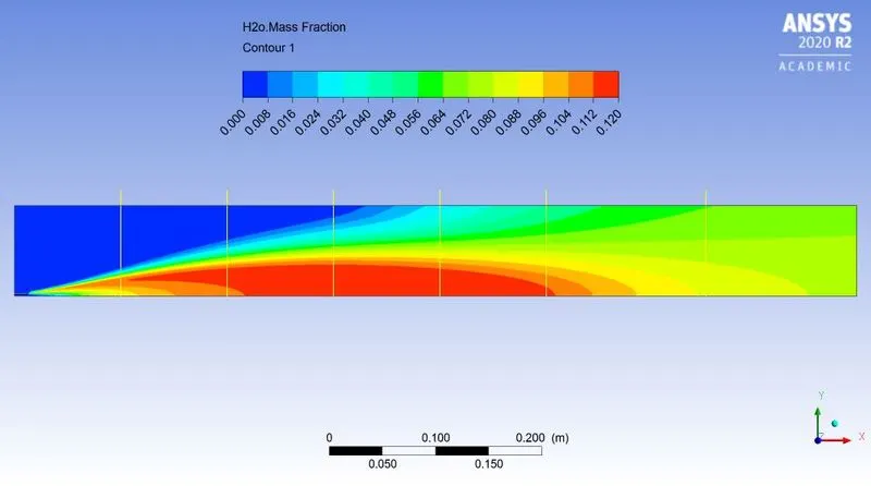
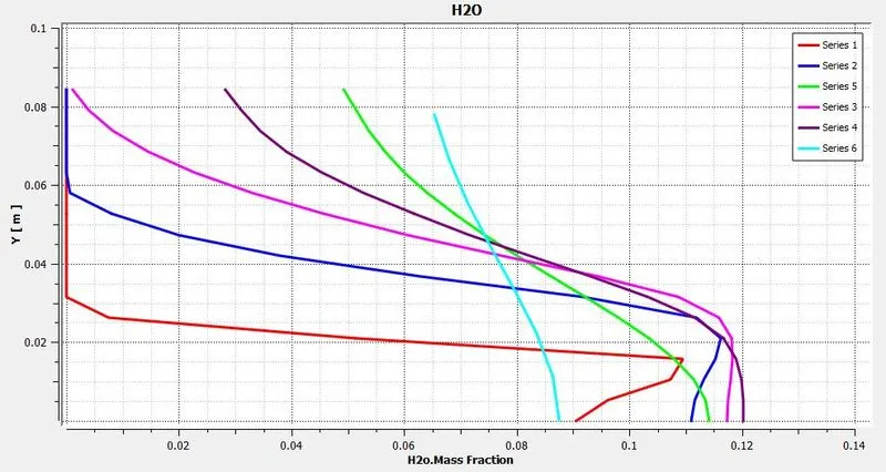
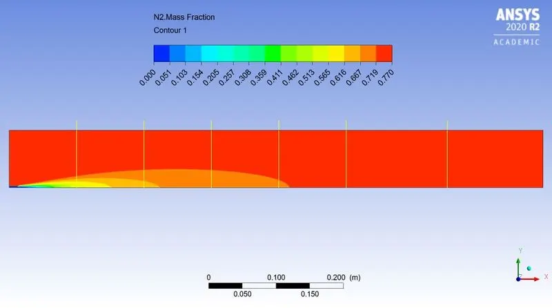
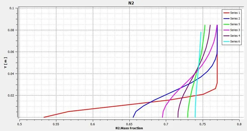
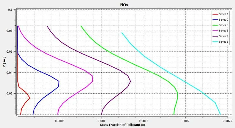
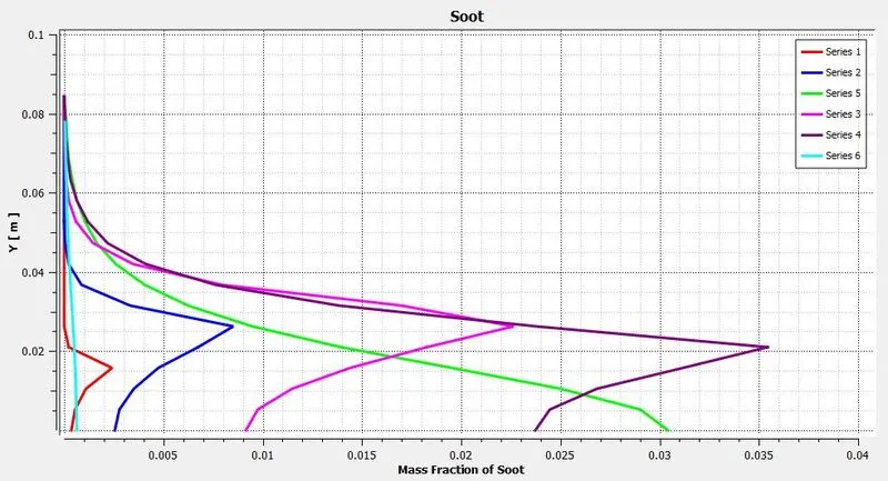
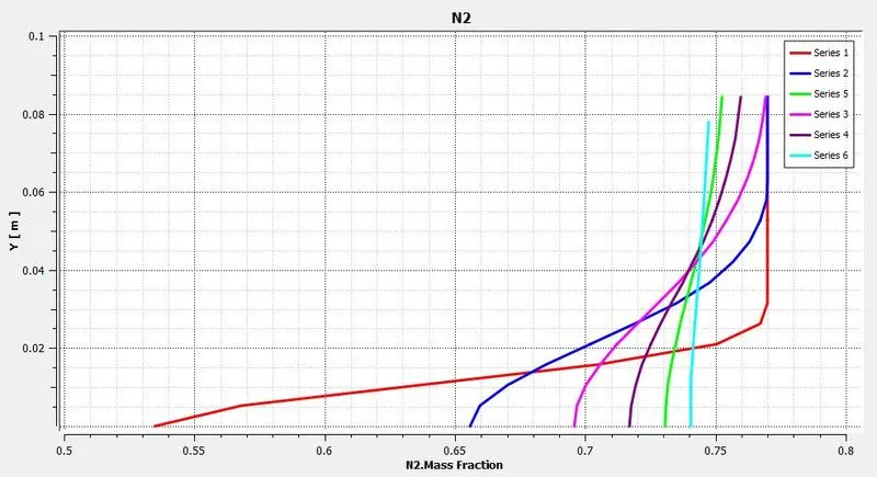
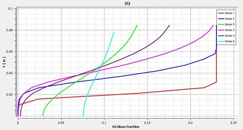
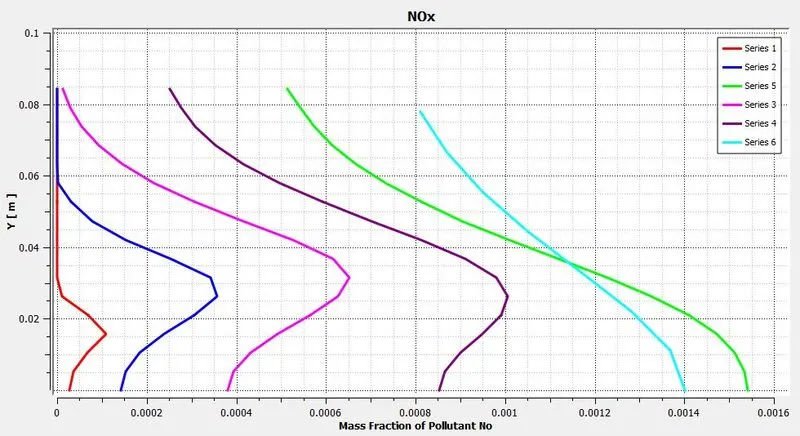
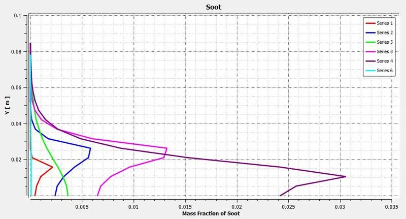
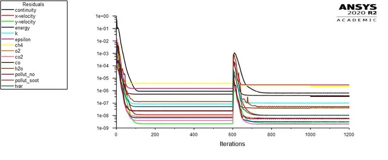
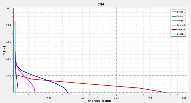
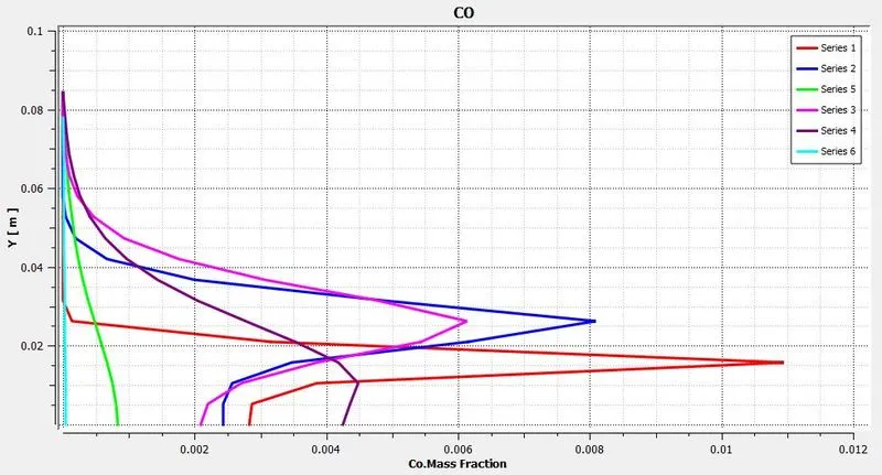
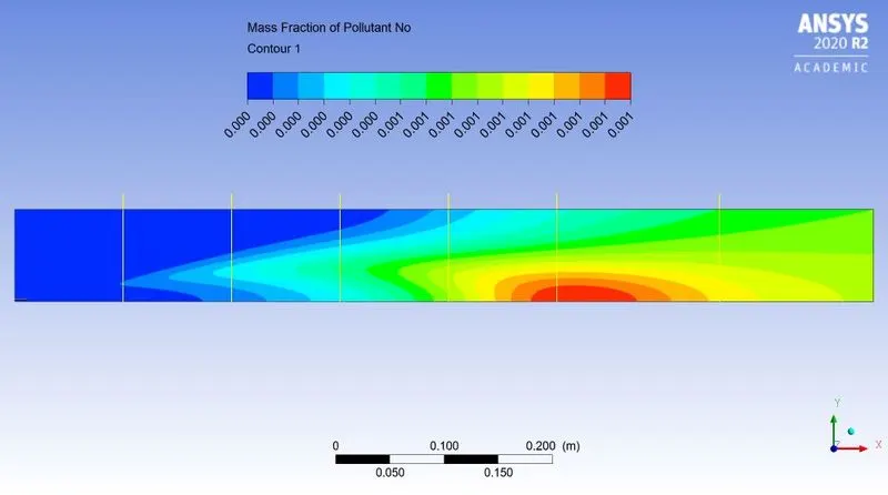
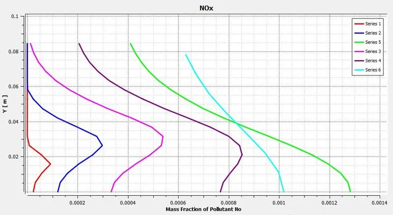
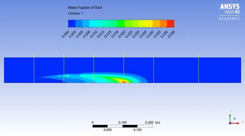
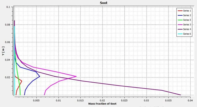
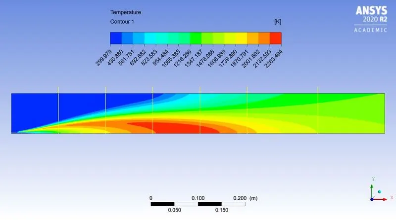
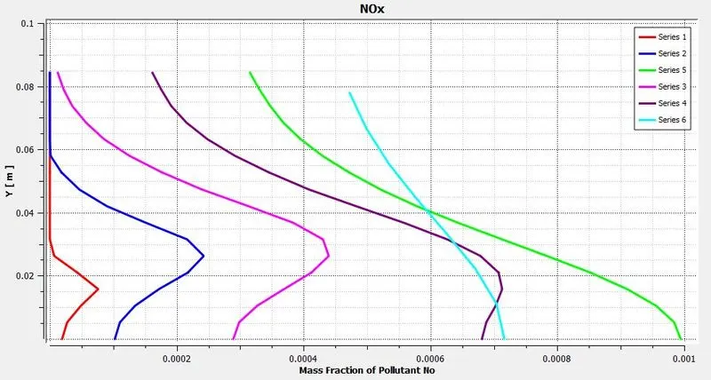
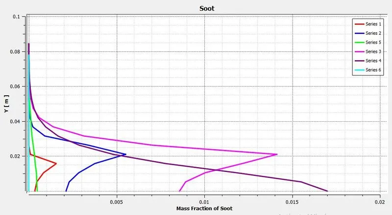
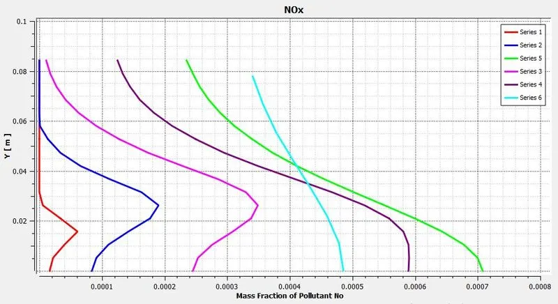
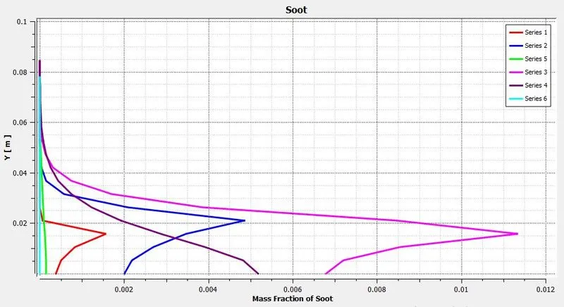
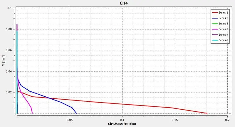
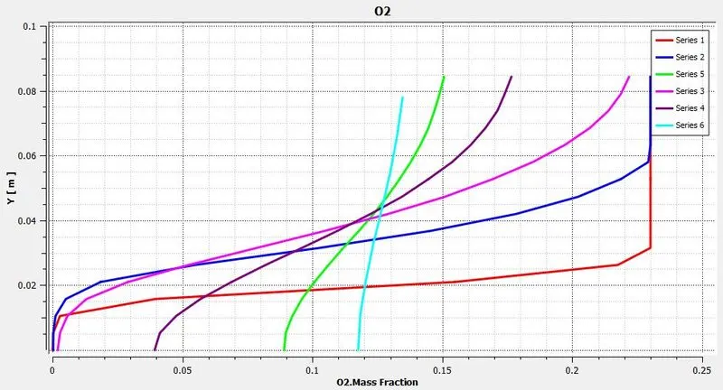
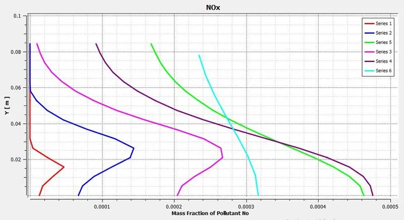
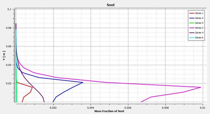
As shown in above figure we have created 6 vertical lines parallel to Y-axis on XY plane. By using line probe ANSYS CFD postprocessor collects data in 20 points on same line. And using that data charts are created.

~Case 1:

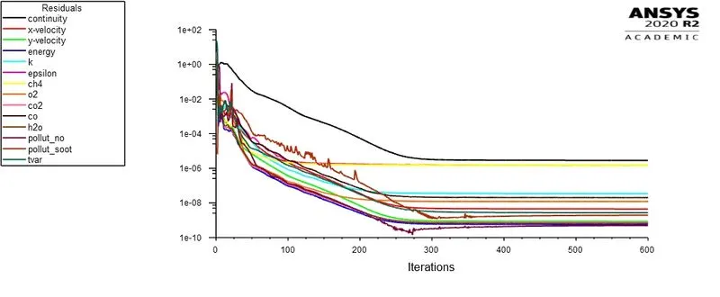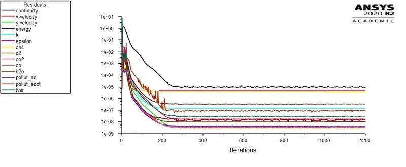
Fig: Residual plot

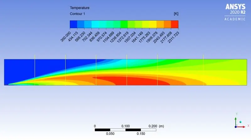
Fig: Temperature contour

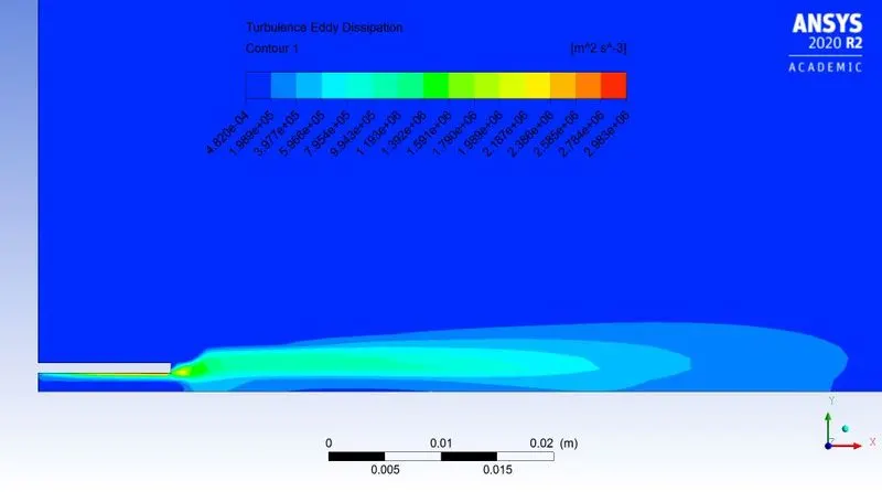
Fig: Turbulence Eddy dissipation contour

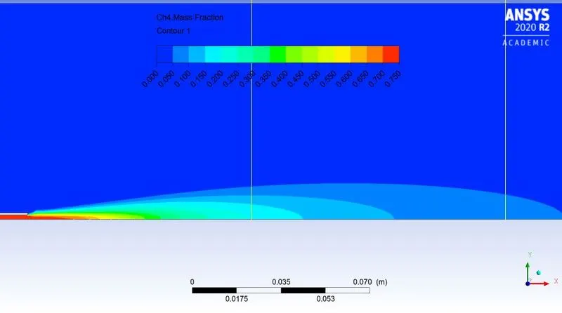
Fig: Mass fraction of `CH_4`

Fig: Mass fraction at various location

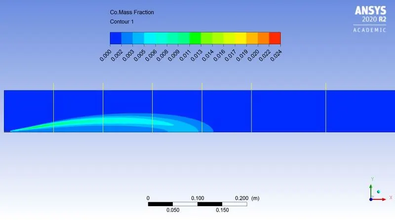
Fig: Mass fraction of `CO`

Fig: Mass fraction at various location

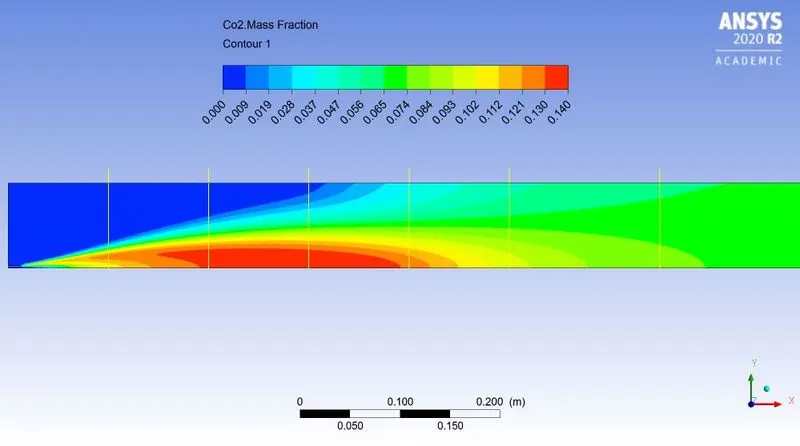
Fig: Mass fraction of `CO_2`

Fig: Mass fraction at various location

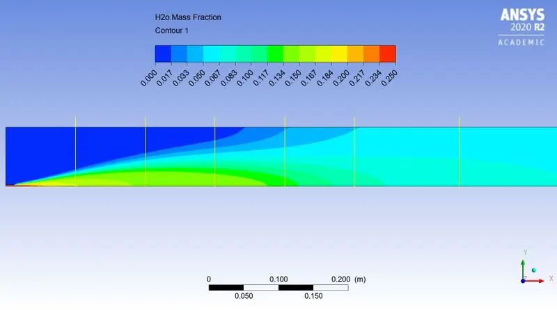
Fig: Mass fraction of `H_2O`

Fig: Mass fraction at various location

Fig: Mass fraction of `N_2`

Fig: Mass fraction at various location

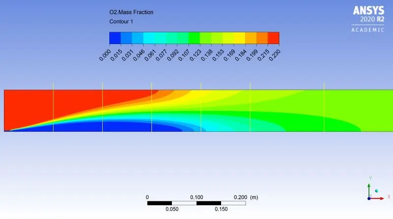
Fig: Mass fraction of `O_2`

Fig: Mass fraction at various location

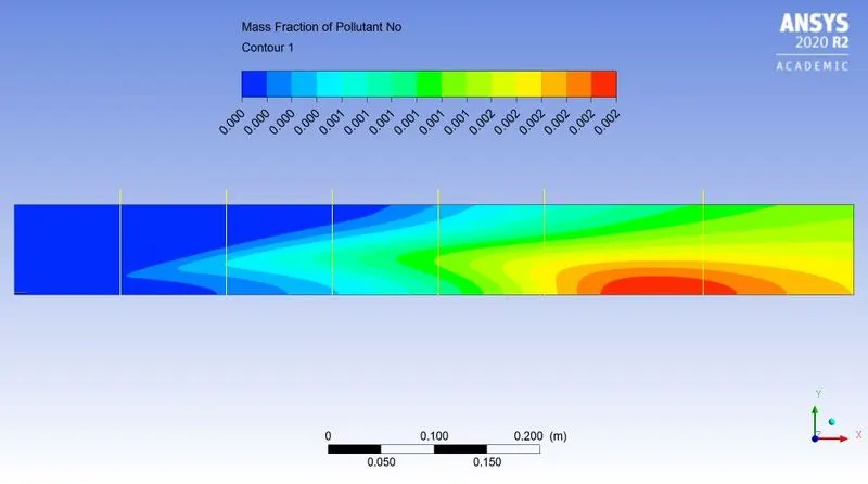
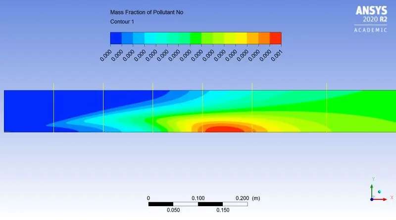
Fig: Mass fraction of `NO_x`

Fig: Mass fraction at various location

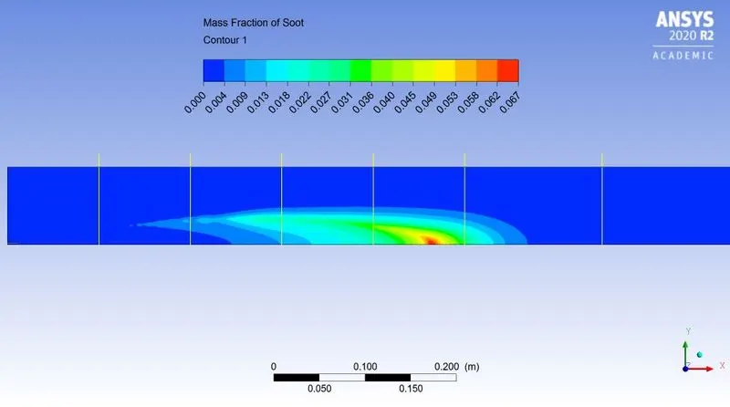
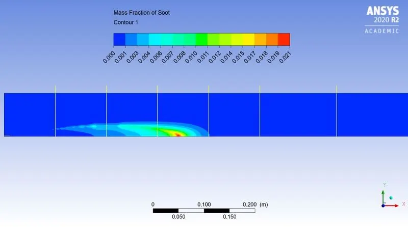
Fig: Mass fraction of `"Soot"`

Fig: Mass fraction at various location

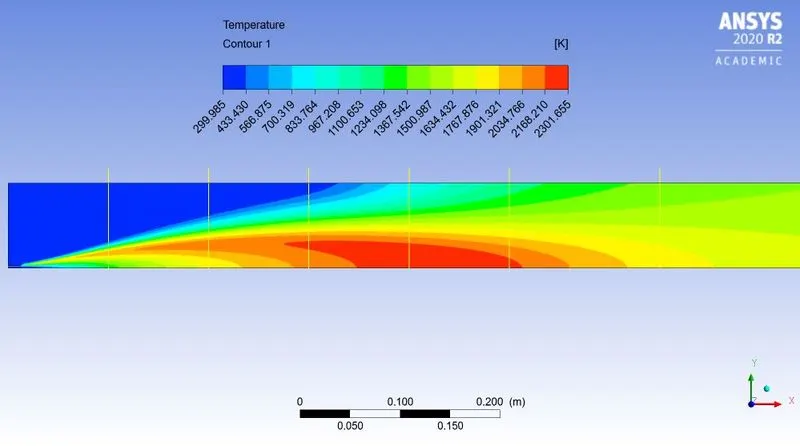
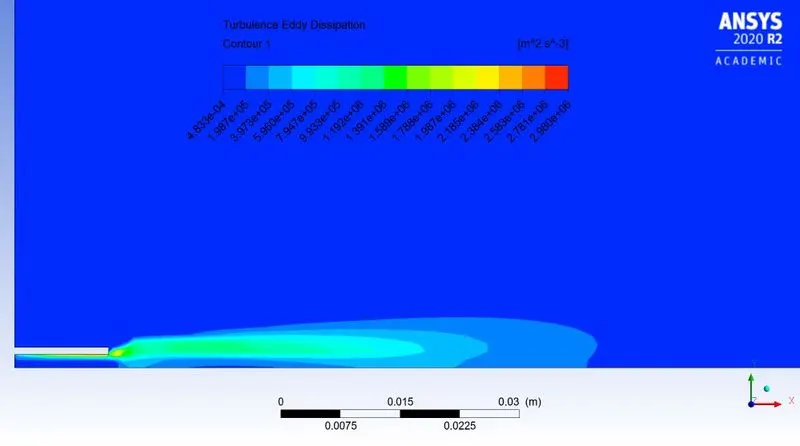
~Case 2.1:

`CH_4 = 95%`

`H_2O = 5%`

Fig: Residual plot
Fig: Temperature contour
Fig: Turbulence Eddy dissipation contour
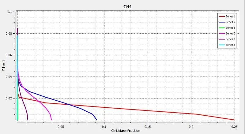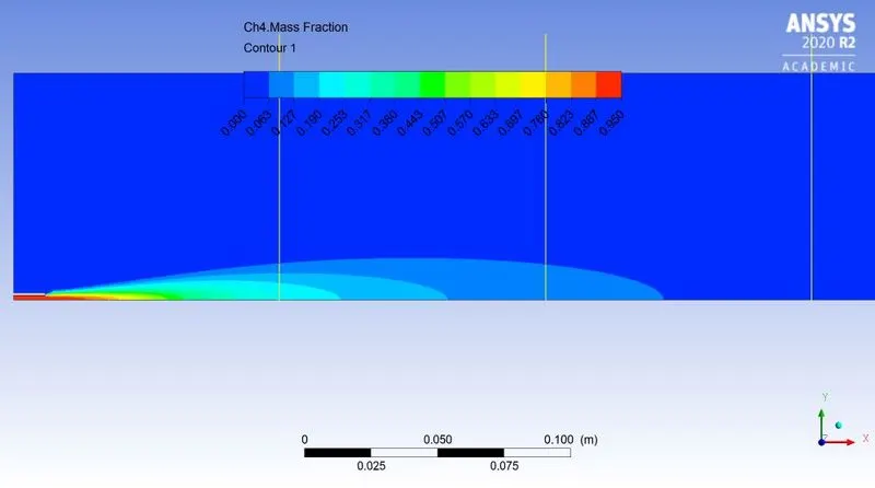
Fig: Mass fraction of `CH_4`	Fig: Mass fraction at various location
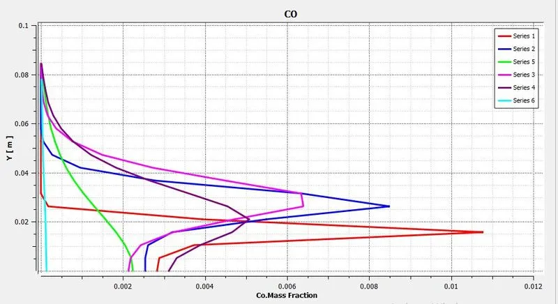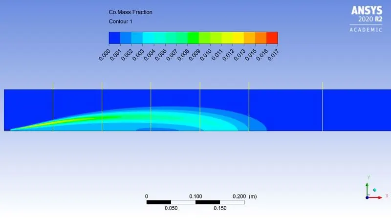
Fig: Mass fraction of `CO`	Fig: Mass fraction at various location
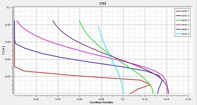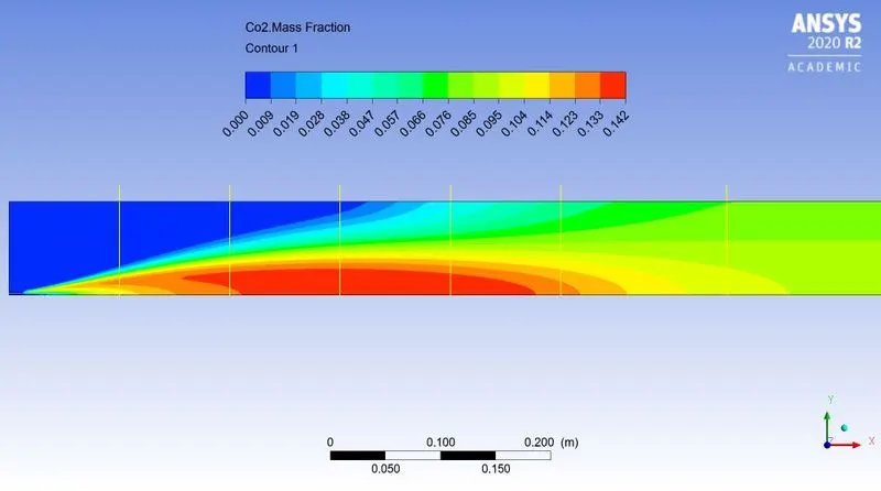
Fig: Mass fraction of `CO_2`	Fig: Mass fraction at various location
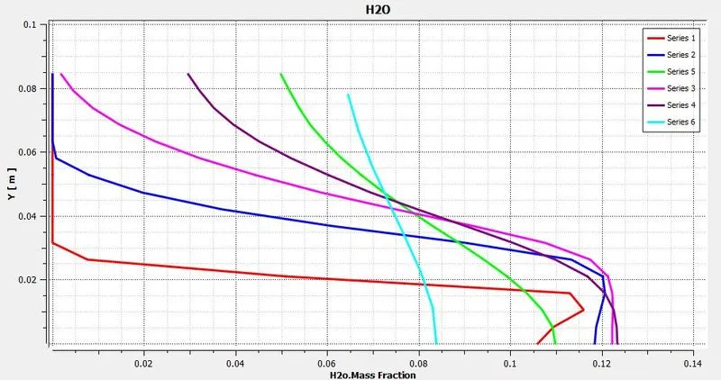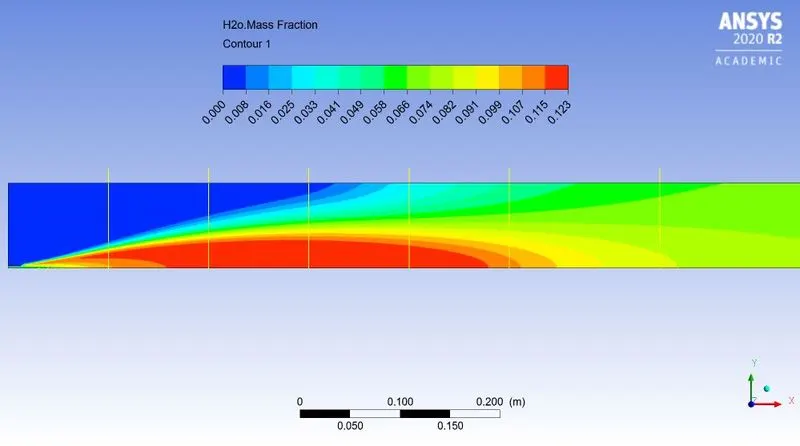
Fig: Mass fraction of `H_2O`	Fig: Mass fraction at various location
Fig: Mass fraction of `N_2`	Fig: Mass fraction at various location
Fig: Mass fraction of `O_2`	Fig: Mass fraction at various location
Fig: Mass fraction of `NO_x`
Fig: Mass fraction at various location
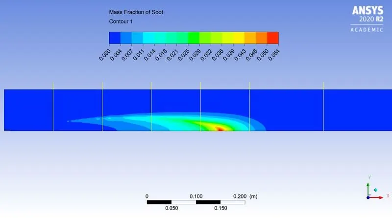
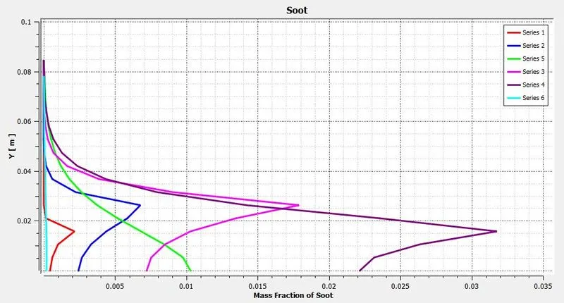
Fig: Mass fraction of `"Soot"`
Fig: Mass fraction at various location

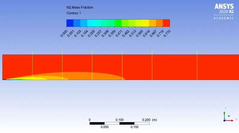
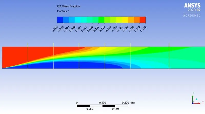
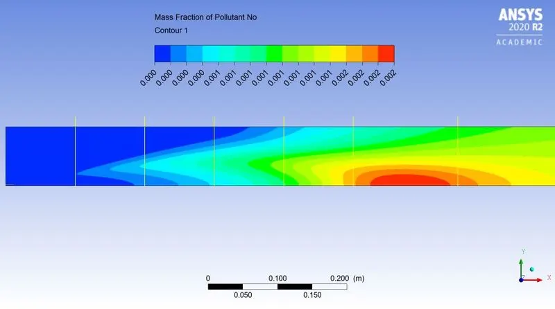
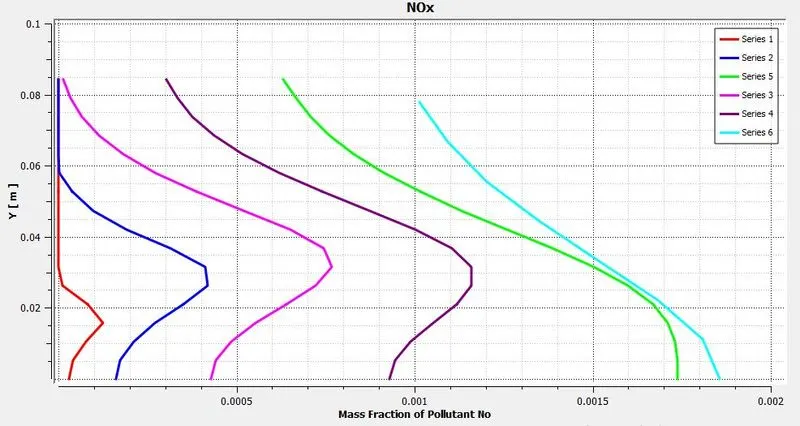
~Case 2.2:

`CH_4 = 90%`

`H_2O = 10%`

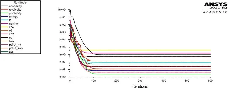
Fig: Residual plot
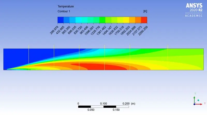
Fig: Temperature contour
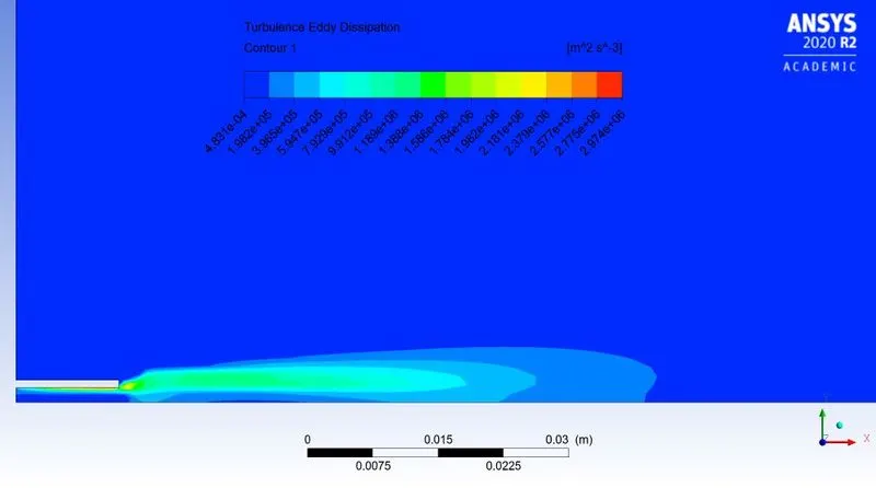
Fig: Turbulence Eddy dissipation contour
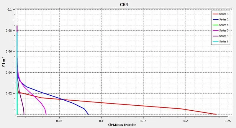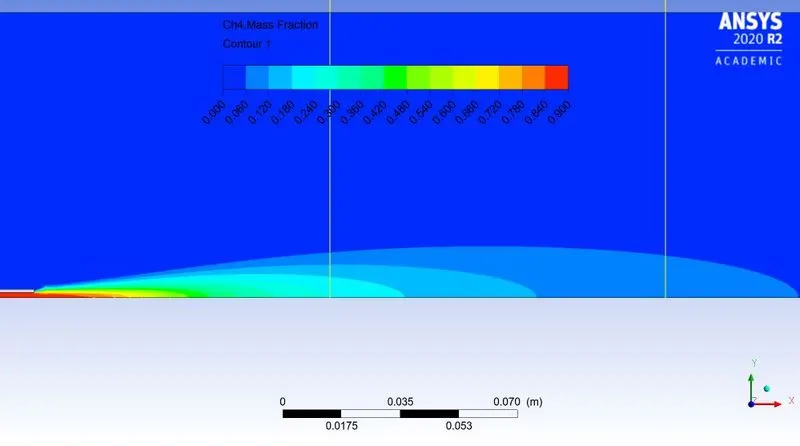
Fig: Mass fraction of `CH_4`	Fig: Mass fraction at various location
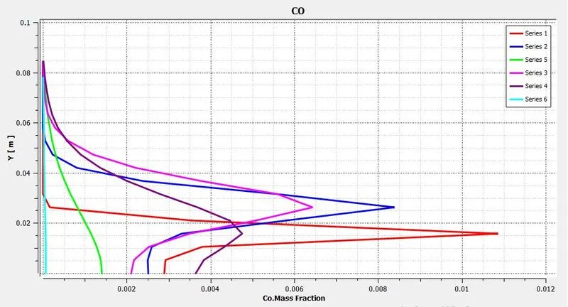Fig: Mass fraction of `CO`	Fig: Mass fraction at various location
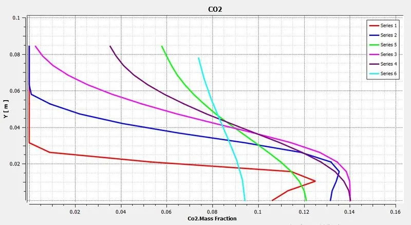Fig: Mass fraction of `CO_2`	Fig: Mass fraction at various location
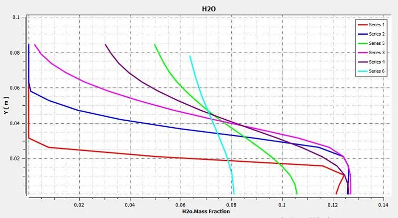Fig: Mass fraction of `H_2O`	Fig: Mass fraction at various location
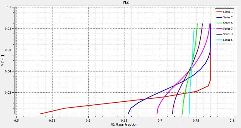Fig: Mass fraction of `N_2`	Fig: Mass fraction at various location
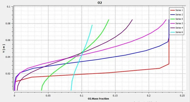Fig: Mass fraction of `O_2`	Fig: Mass fraction at various location
Fig: Mass fraction of `NO_x`
Fig: Mass fraction at various location
Fig: Mass fraction of `"Soot"`
Fig: Mass fraction at various location

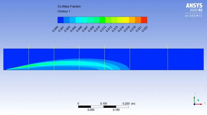
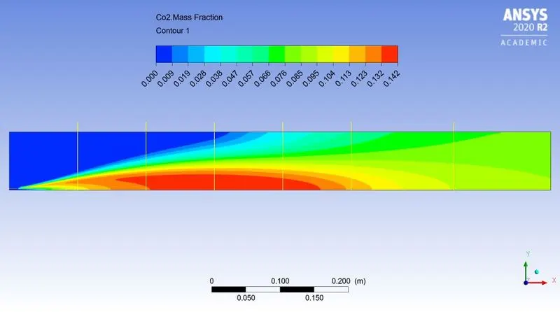
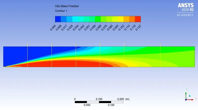
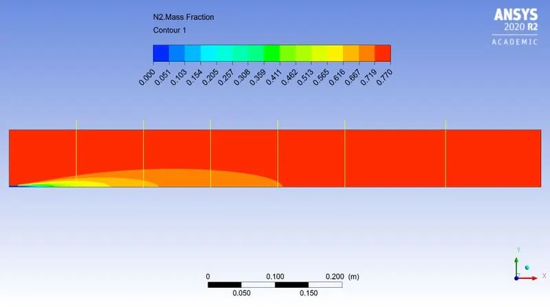
~Case 2.3:

`CH_4 = 85%`

`H_2O = 15%`

Fig: Residual plot
Fig: Temperature contour
Fig: Turbulence Eddy dissipation contour
Fig: Mass fraction of `CH_4`	Fig: Mass fraction at various location
Fig: Mass fraction of `CO`	Fig: Mass fraction at various location
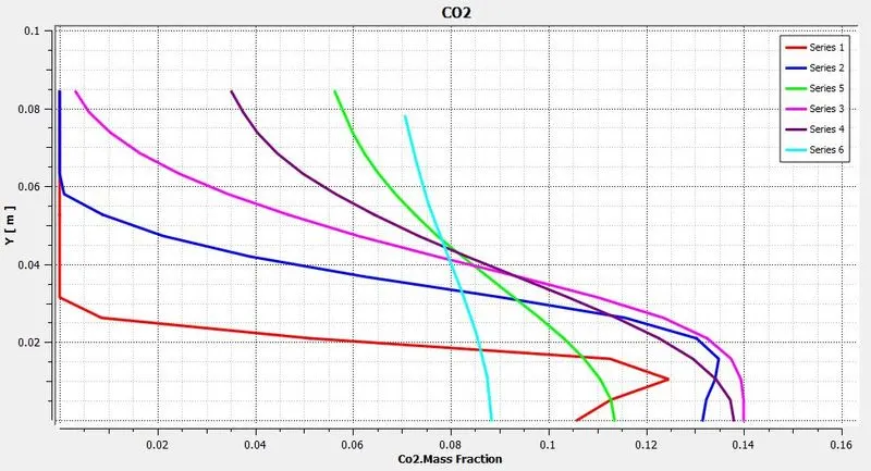Fig: Mass fraction of `CO_2`	Fig: Mass fraction at various location
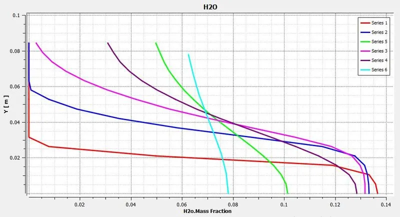Fig: Mass fraction of `H_2O`	Fig: Mass fraction at various location
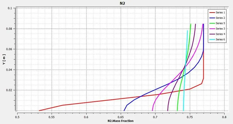Fig: Mass fraction of `N_2`	Fig: Mass fraction at various location
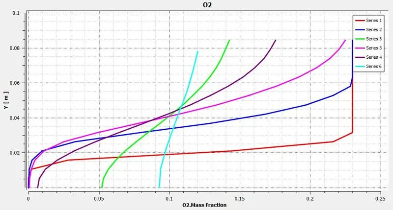Fig: Mass fraction of `O_2`	Fig: Mass fraction at various location
Fig: Mass fraction of `NO_x`
Fig: Mass fraction at various location
Fig: Mass fraction of `"Soot"`
Fig: Mass fraction at various location

~Case 2.4:

`CH_4 = 80%`

`H_2O = 20%`

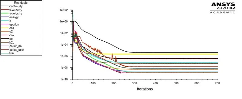Fig: Residual plot
Fig: Temperature contour
Fig: Turbulence Eddy dissipation contour
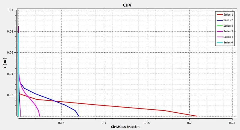Fig: Mass fraction of `CH_4`	Fig: Mass fraction at various location
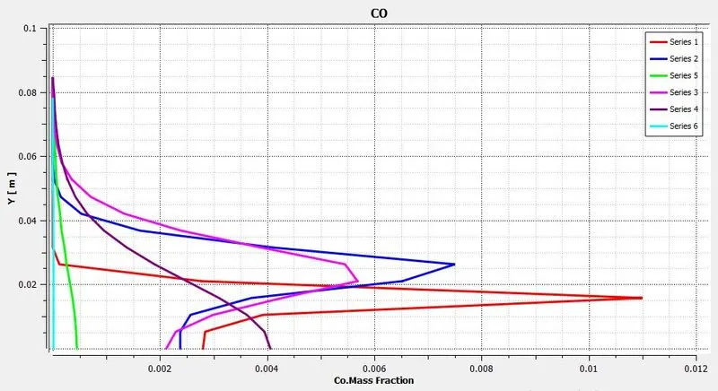Fig: Mass fraction of `CO`	Fig: Mass fraction at various location
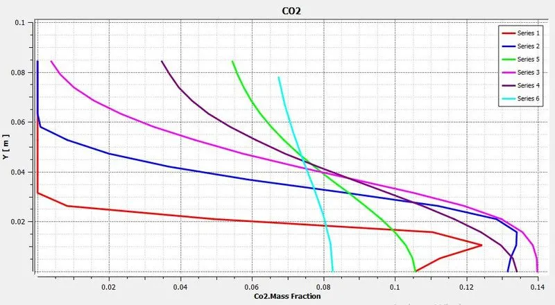Fig: Mass fraction of `CO_2`	Fig: Mass fraction at various location
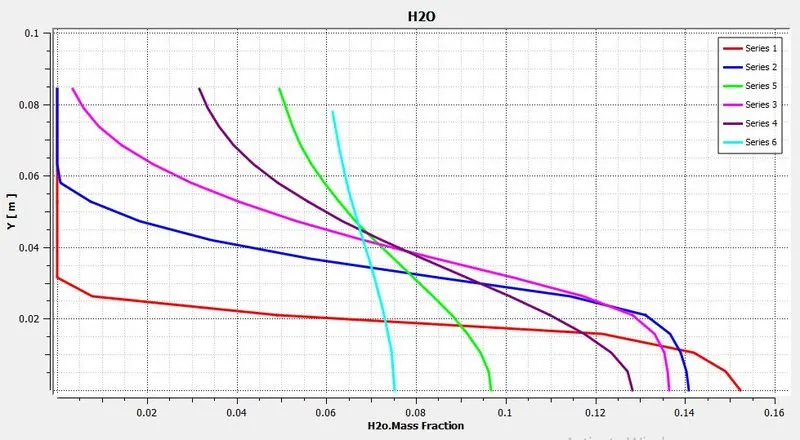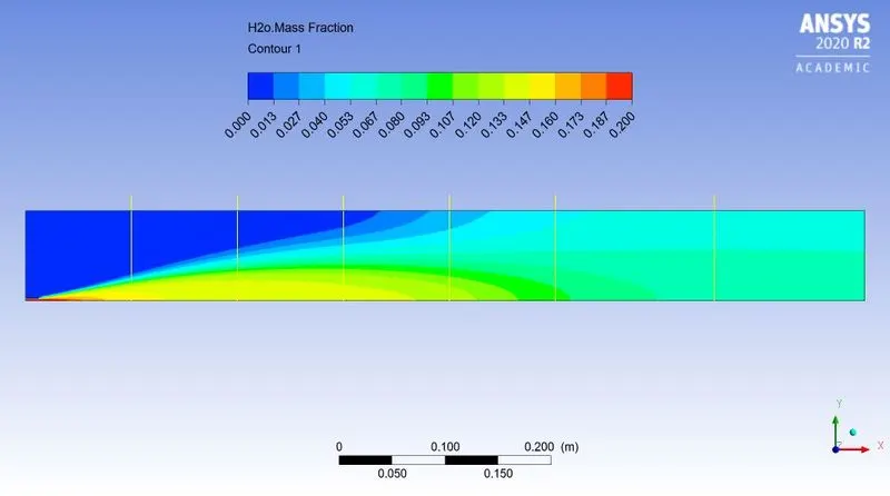
Fig: Mass fraction of `H_2O`	Fig: Mass fraction at various location
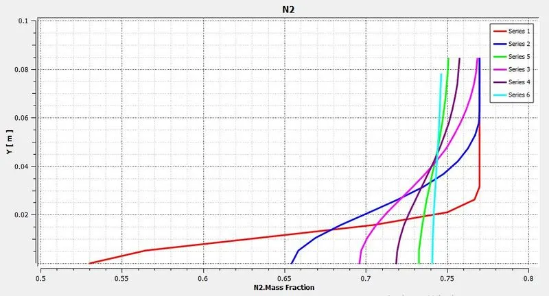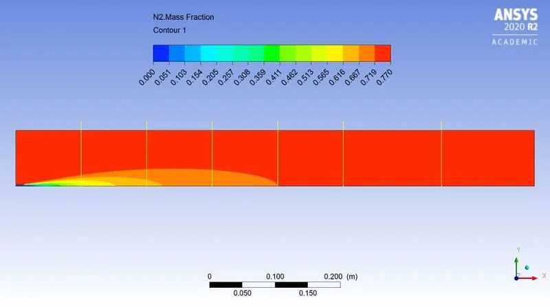
Fig: Mass fraction of `N_2`	Fig: Mass fraction at various location
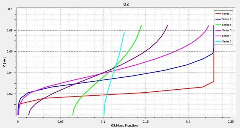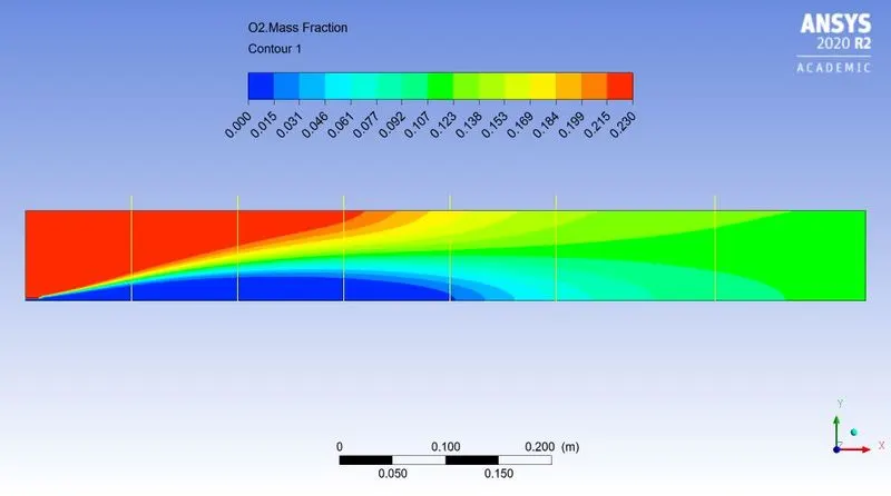
Fig: Mass fraction of `O_2`	Fig: Mass fraction at various location
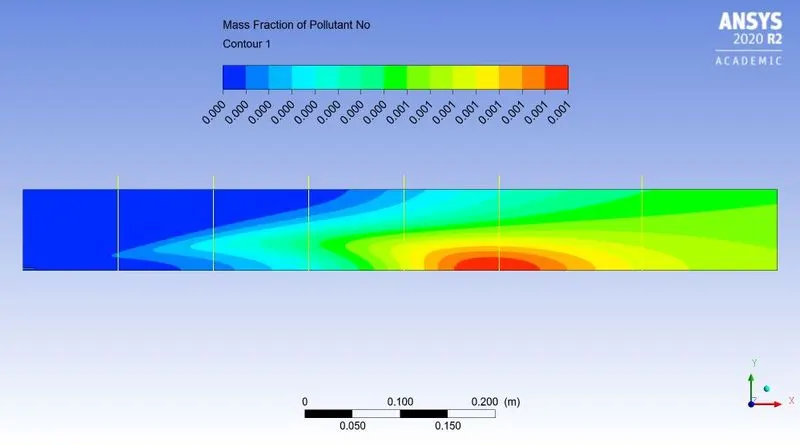
Fig: Mass fraction of `NO_x`
Fig: Mass fraction at various location
Fig: Mass fraction of `"Soot"`
Fig: Mass fraction at various location

~Case 2.5:

`CH_4 = 75%`

`H_2O = 25%`

Fig: Residual plot
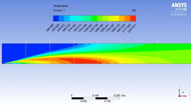
Fig: Temperature contour
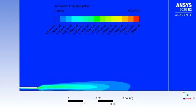
Fig: Turbulence Eddy dissipation contour
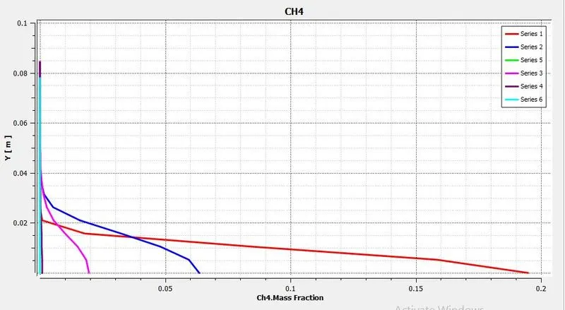Fig: Mass fraction of `CH_4`	Fig: Mass fraction at various location
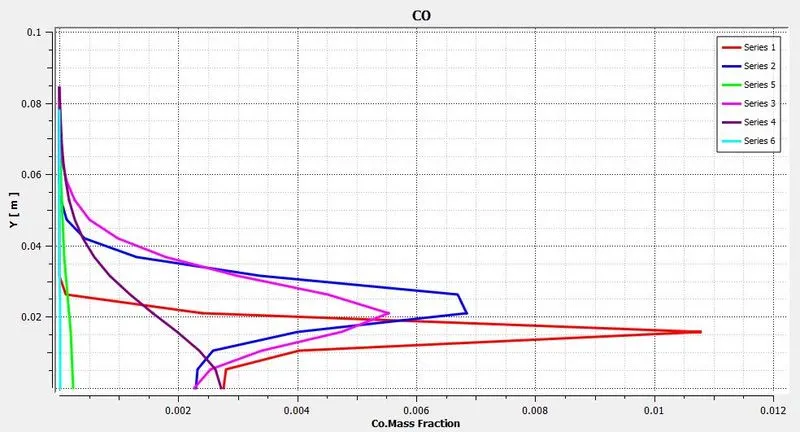Fig: Mass fraction of `CO`	Fig: Mass fraction at various location
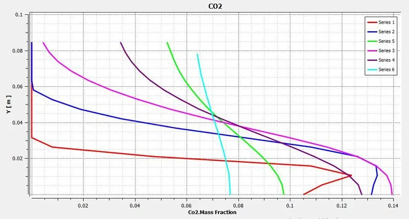Fig: Mass fraction of `CO_2`	Fig: Mass fraction at various location
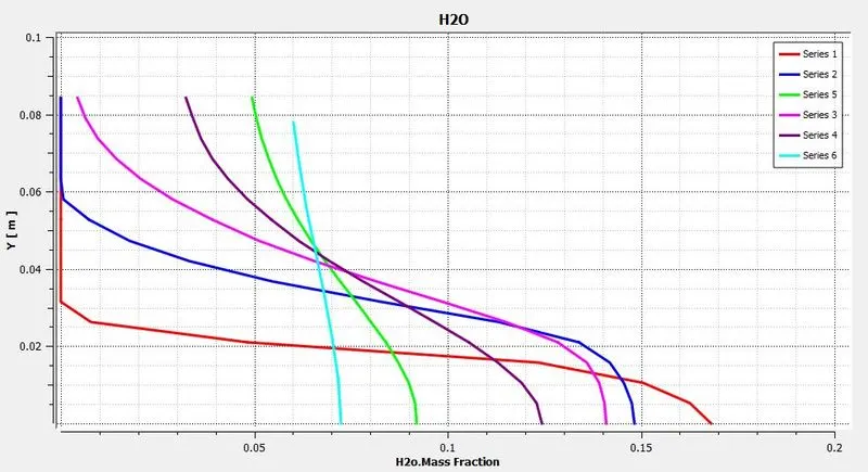Fig: Mass fraction of `H_2O`	Fig: Mass fraction at various location
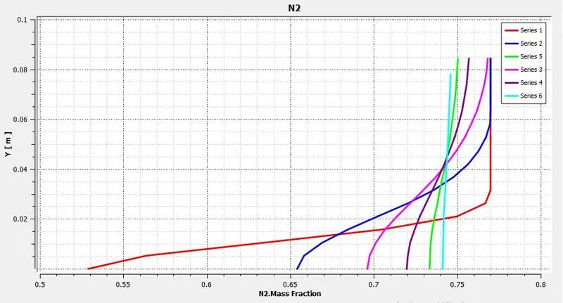Fig: Mass fraction of `N_2`	Fig: Mass fraction at various location
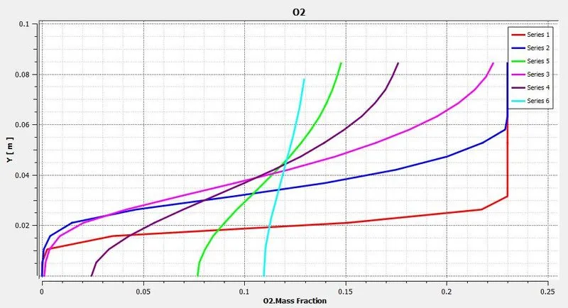Fig: Mass fraction of `O_2`	Fig: Mass fraction at various location
Fig: Mass fraction of `NO_x`
Fig: Mass fraction at various location
Fig: Mass fraction of `"Soot"`
Fig: Mass fraction at various location

~Case 2.6:

`CH_4 = 70%`

`H_2O = 30%`

Fig: Residual plot
Fig: Temperature contour
Fig: Turbulence Eddy dissipation contour
Fig: Mass fraction of `CH_4`	Fig: Mass fraction at various location
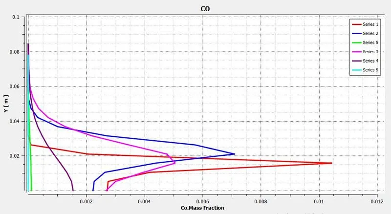Fig: Mass fraction of `CO`	Fig: Mass fraction at various location
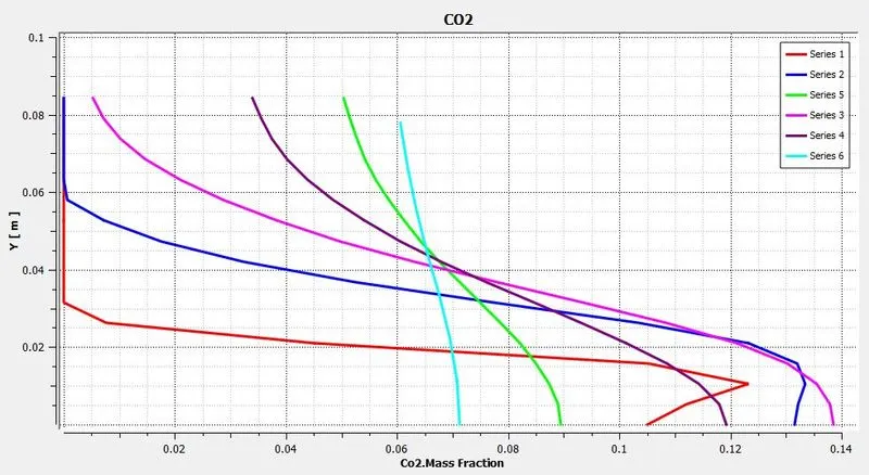Fig: Mass fraction of `CO_2`	Fig: Mass fraction at various location
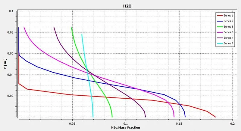Fig: Mass fraction of `H_2O`	Fig: Mass fraction at various location
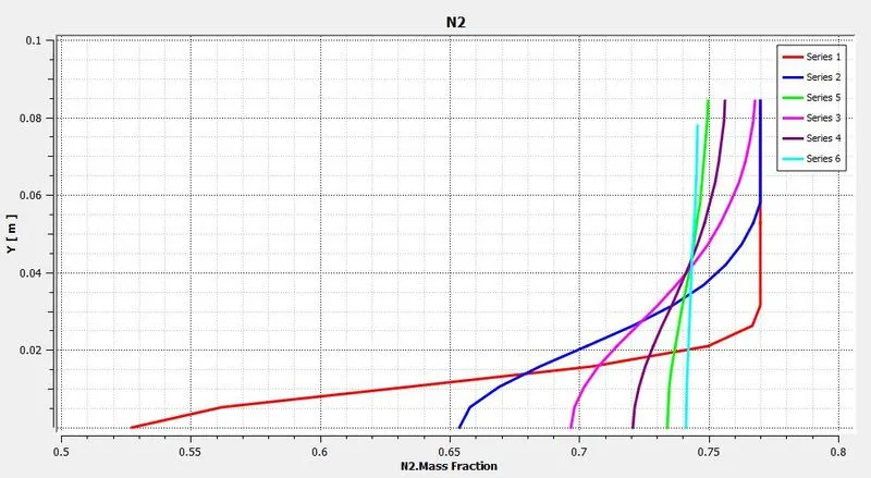Fig: Mass fraction of `N_2`	Fig: Mass fraction at various location
Fig: Mass fraction of `O_2`	Fig: Mass fraction at various location
Fig: Mass fraction of `NO_x`
Fig: Mass fraction at various location
Fig: Mass fraction of `"Soot"`
Fig: Mass fraction at various location

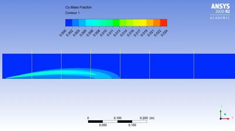
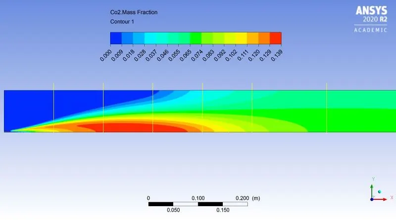
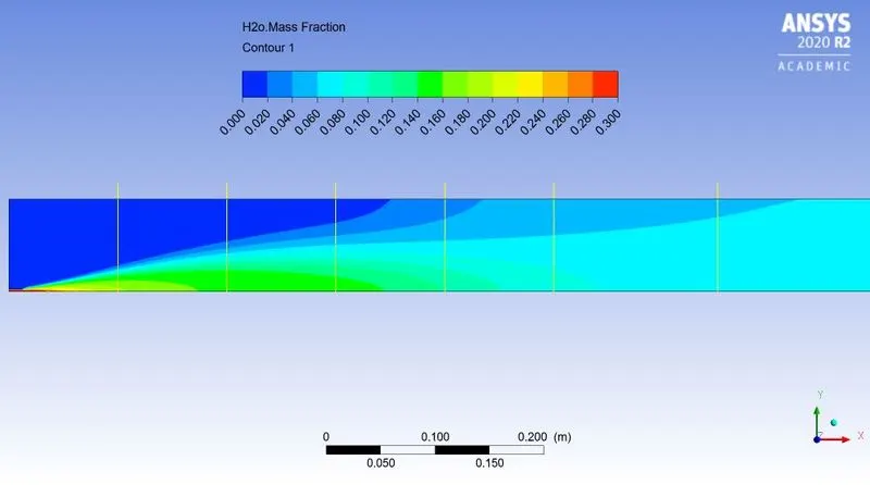
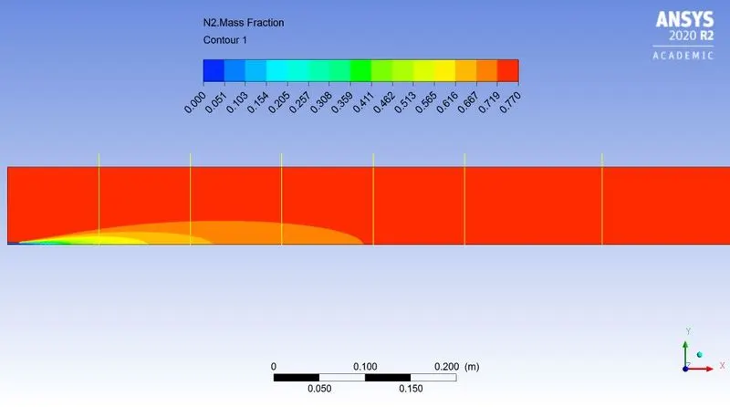
Result:-

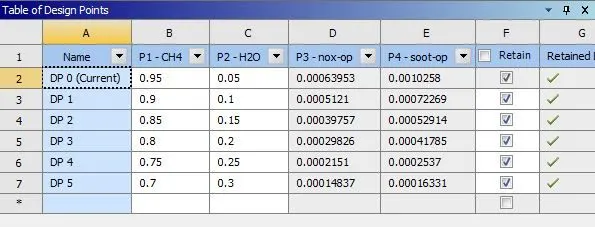Fig: Parametric study approach to obtain result

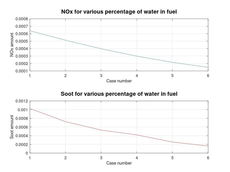
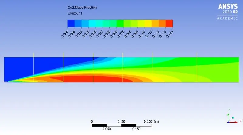
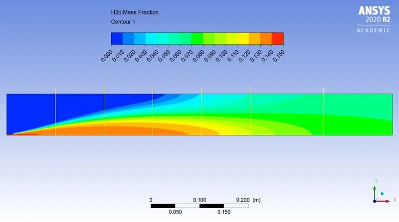
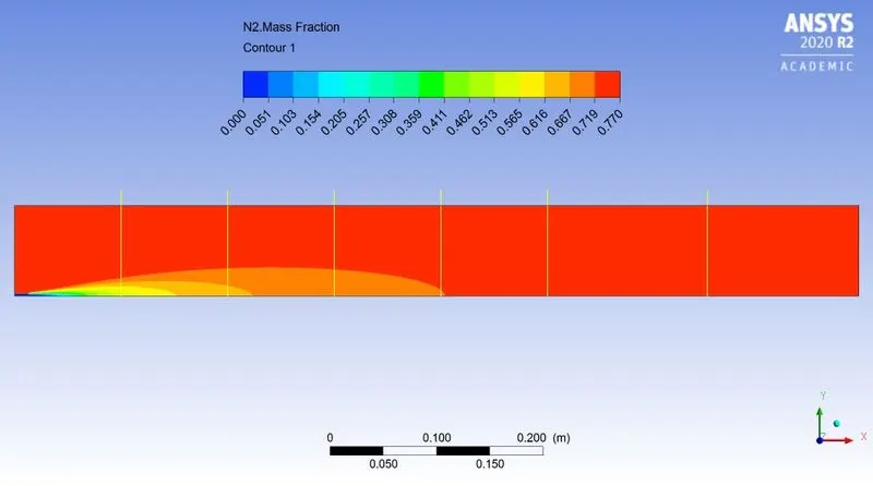
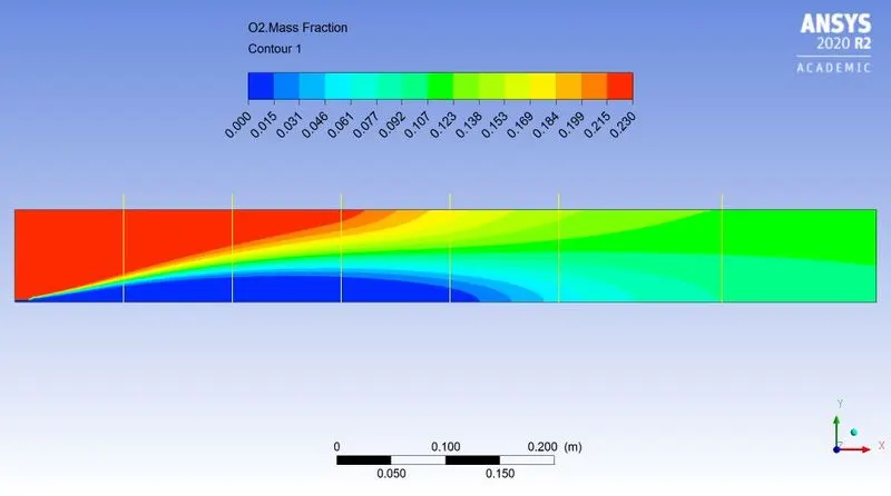
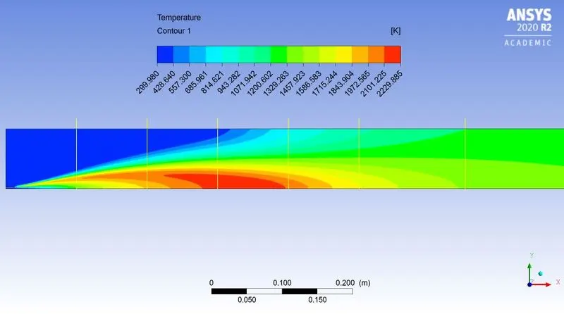
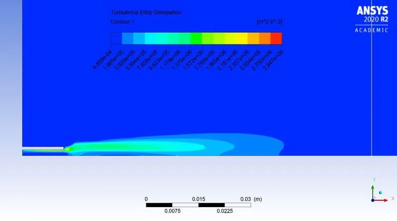
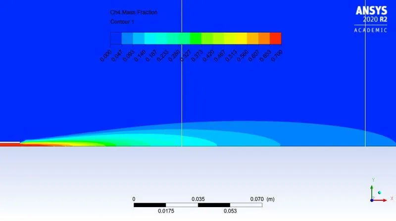
Conclusion:- From observing above post processed data, plots and results we can conclude that-

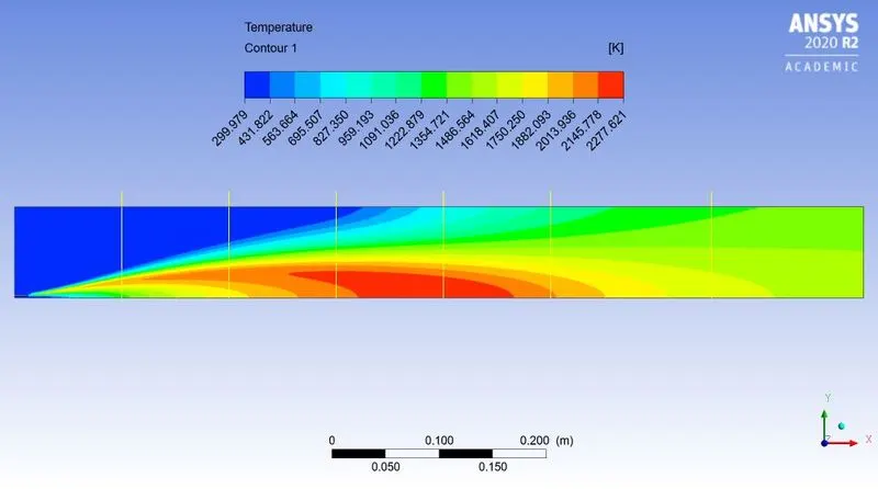
1. Temperature gradually decreases as water content increases in fuel
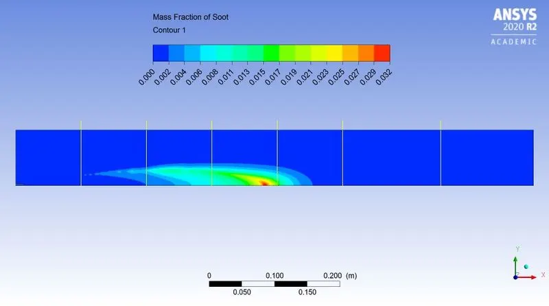
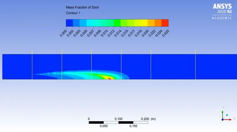
2. Addition of water content in fuel results decreased in soot formation. It happens due to oxygen molecule from water which reacts with unburnt fuel and soot particles decreases.
3. Addition of water results decreased in formation.
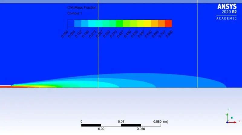
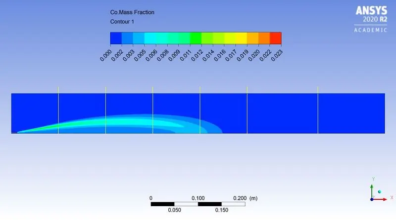
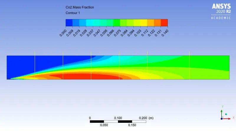
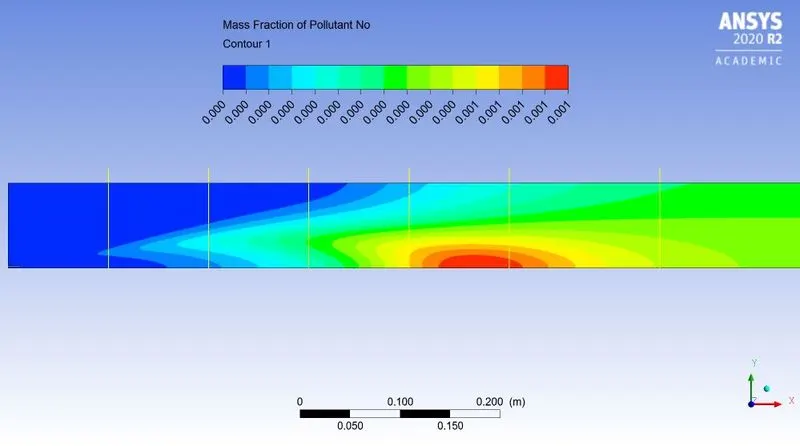
4. The pollutant like `NO_x` & Soot mass fraction is more near outlet.
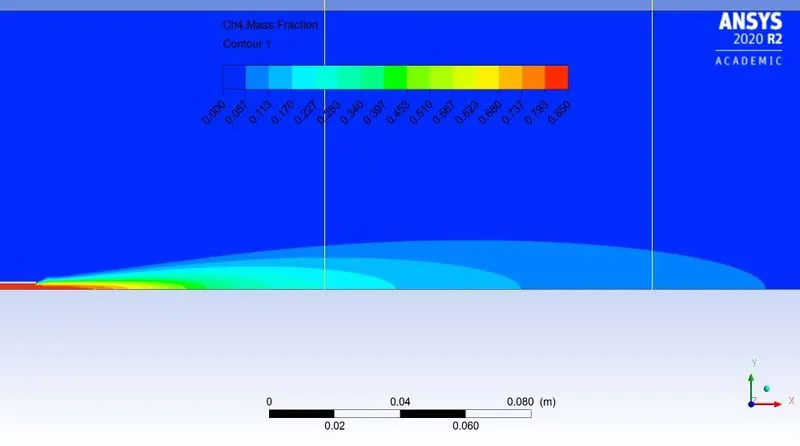
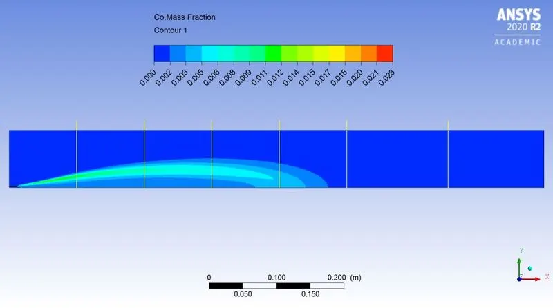
5. As water is added in fuel, the large amount of pollutant generates nearer to inlet.
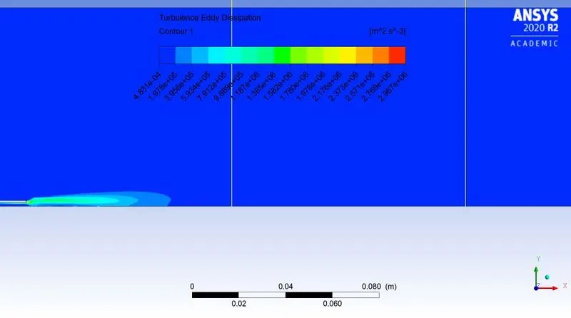
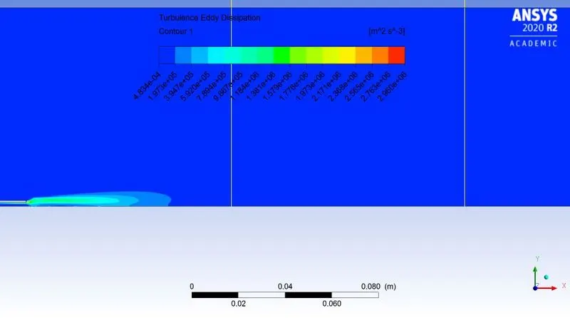
6. The ignition happens due to turbulence and eddy dissipation.