Assignment 4
AIM:
To run the simulation and compare the simulations of Failure Johnsons(4 cases) and Law 36 and Law 27 by changing the properties.
ABSTRACT:
To change the material properties with respect to the cases and run the simulation in hypermesh in Radioss block by assigning the required values and then to run the crash animation in Hyperview block and Plotting graphs in HyperGraph 2D block with different energies and then comparing with different cases.
METHODOLOGY:
- Hypermesh>Analysis>Radioss to convert the file format to Radioss.
- Hyperview to run the animation of crash into a rigidwall.
- HyperGraph 2D to plot the graphs.
PROCEDURE:
CASE 1:
1.Import the Failure_Johnson Starter file(0000.rad) from Solver deck.
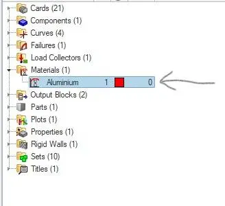
2.Change the material name as ‘Law2_epsmax_failure’ from ‘Aluminium’ and run the simulation as it is.
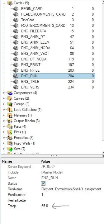
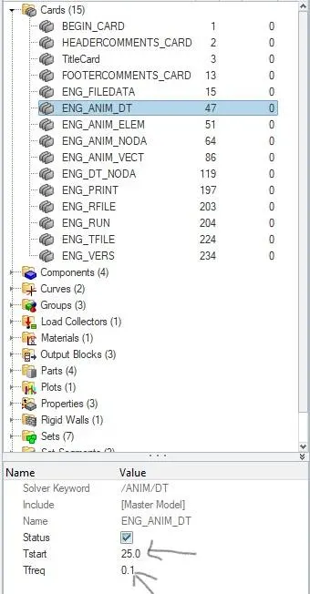
3.As a choice can assign the value of Tstop as 55ms in Cards>Engine Run and in Engine-Animation-DT,Tstart as 0 and Tfreq is 0.1.
4.In Analysis>Radioss,give the input file as (0000.rad) file and ‘tick’ include connectors which keeps in connected the surfaces and option as ‘-nt 4’ and click ‘Radioss’.

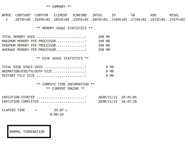
5.It runs the base simulation and gives the error file as (0001.out) file which consists of mass error,energy error,external work and at the end of file it should indicate ‘NORMAL TERMINATION’ which indicates successful simulation without any errors.
6.Now change the Client selector (ToolBar) from ‘Hypermesh’ to ‘HyperView’ to create the animation of crash.Upload the file (h3d) in ‘Load model and results’ of case 1 and ‘Apply’.Save the animation video.
7.Now change the Client selector from ‘Hyperview’ to ‘HyperGraph 2D’ where you need to plot the graphs which are given.
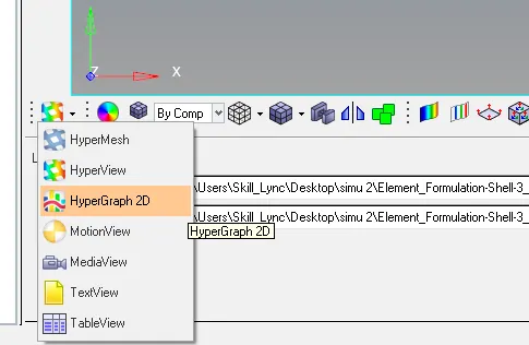
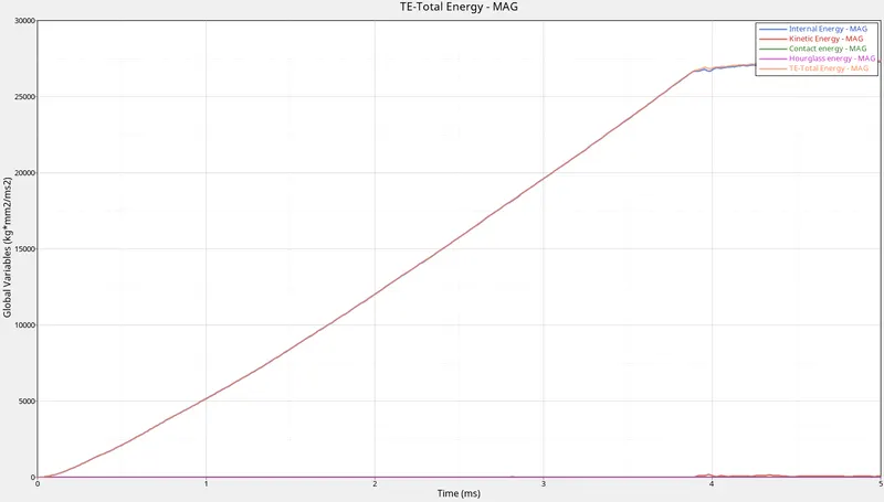
8.Plot the graphs for kinetic energy, internal energy, hourglass energy, contact energy, total energy of the simulations.
CASE 2:
1.Import the Failure_Johnson Starter file(0000.rad) from Solver deck.
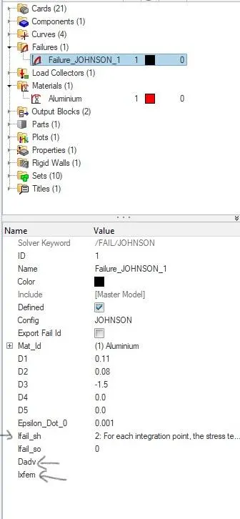
2.Now assign the values of ‘Ifail_sh=1,Dadv=1 and Ixfem=1’ in the failures of /Failure/JOHNSON card and name the material to ‘Law2_epsmax_crack’ from ‘Aluminium’.
3.As a choice can assign the value of Tstop as 55ms in Cards>Engine Run and in Engine-Animation-DT,Tstart as 0 and Tfreq is 0.1.
4.In Analysis>Radioss,give the input file as (0000.rad) file and ‘tick’ include connectors which keeps in connected the surfaces and option as ‘-nt 4’ and click ‘Radioss’.
5.It runs the base simulation and gives the error file as (0001.out) file which consists of mass error,energy error,external work and at the end of file it should indicate ‘NORMAL TERMINATION’ which indicates successful simulation without any errors.
6.Now change the Client selector (ToolBar) from ‘Hypermesh’ to ‘HyperView’ to create the animation of crash.Upload the file (h3d) in ‘Load model and results’ of case 1 and ‘Apply’.Save the animation video.
7.Now change the Client selector from ‘Hyperview’ to ‘HyperGraph 2D’ where you need to plot the graphs which are given.
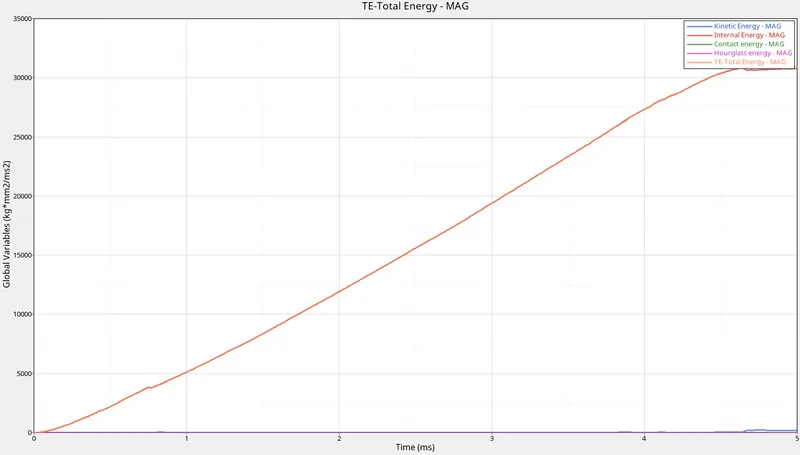
8.Plot the graphs for kinetic energy, internal energy, hourglass energy, contact energy, total energy of the simulations.
CASE 3:
1.Import the Failure_Johnson Starter file(0000.rad) from Solver deck.
2.Delete the /Failure/JOHNSON card and name the material as ‘Law2_epsmax_nofail’.
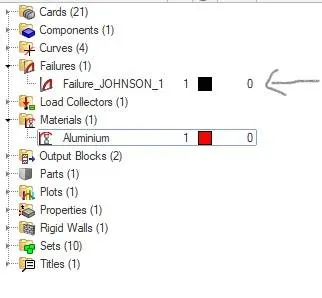
3.As a choice can assign the value of Tstop as 55ms in Cards>Engine Run and in Engine-Animation-DT,Tstart as 0 and Tfreq is 0.1.
4.In Analysis>Radioss,give the input file as (0000.rad) file and ‘tick’ include connectors which keeps in connected the surfaces and option as ‘-nt 4’ and click ‘Radioss’.
5.It runs the base simulation and gives the error file as (0001.out) file which consists of mass error,energy error,external work and at the end of file it should indicate ‘NORMAL TERMINATION’ which indicates successful simulation without any errors.
6.Now change the Client selector (ToolBar) from ‘Hypermesh’ to ‘HyperView’ to create the animation of crash.Upload the file (h3d) in ‘Load model and results’ of case 1 and ‘Apply’.Save the animation video.
7.Now change the Client selector from ‘Hyperview’ to ‘HyperGraph 2D’ where you need to plot the graphs which are given.
8.Plot the graphs for kinetic energy, internal energy, hourglass energy, contact energy, total energy of the simulations.
CASE 4:
1.Import the Failure_Johnson Starter file(0000.rad) from Solver deck.
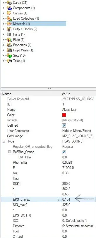
2.Now delete the EPS_p_max value as it was 0.151 and change to 0 in material card and name the material as ‘Law 2’.
3.As a choice can assign the value of Tstop as 55ms in Cards>Engine Run and in Engine-Animation-DT,Tstart as 0 and Tfreq is 0.1.
4.InAnalysis>Radioss,give the input file as (0000.rad) file and ‘tick’ include connectors which keeps in connected the surfaces and option as ‘-nt 4’ and click ‘Radioss’.
5.It runs the base simulation and gives the error file as (0001.out) file which consists of mass error,energy error,external work and at the end of file it should indicate ‘NORMAL TERMINATION’ which indicates successful simulation without any errors.
6.Now change the Client selector (ToolBar) from ‘Hypermesh’ to ‘HyperView’ to create the animation of crash.Upload the file (h3d) in ‘Load model and results’ of case 1 and ‘Apply’.Save the animation video.
7.Now change the Client selector from ‘Hyperview’ to ‘HyperGraph 2D’ where you need to plot the graphs which are given.
8.Plot the graphs for kinetic energy, internal energy, hourglass energy, contact energy, total energy of the simulations.
CASE 5:
1.Import the Failure_Johnson Starter file(0000.rad) from Solver deck.
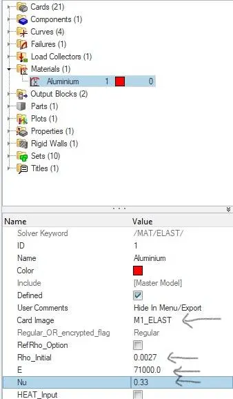
2.Convert the card image from ‘M2_PLAS_JOHN_ZERIL’ (Law 2) to M1_ELAST’ (Law 1) and assign the same values of Density (Rho),Youngs Modulus(E) and Poissons ratio(Nu) in Law 2 to Law 1 as rho=0.0027,E=71000 and Nu=0.33.
3.As a choice can assign the value of Tstop as 55ms in Cards>Engine Run and in Engine-Animation-DT,Tstart as 0 and Tfreq is 0.1.
4.In Analysis>Radioss,give the input file as (0000.rad) file and ‘tick’ include connectors which keeps in connected the surfaces and option as ‘-nt 4’ and click ‘Radioss’.
5.It runs the base simulation and gives the error file as (0001.out) file which consists of mass error,energy error,external work and at the end of file it should indicate ‘NORMAL TERMINATION’ which indicates successful simulation without any errors.
6.Now change the Client selector (ToolBar) from ‘Hypermesh’ to ‘HyperView’ to create the animation of crash.Upload the file (h3d) in ‘Load model and results’ of case 1 and ‘Apply’.Save the animation video.
7.Now change the Client selector from ‘Hyperview’ to ‘HyperGraph 2D’ where you need to plot the graphs which are given.
8.Plot the graphs for kinetic energy, internal energy, hourglass energy, contact energy, total energy of the simulations.
CASE 6:
1.Import the Failure_Johnson Starter file(0000.rad) from Solver deck.
2..Convert the card image from ‘M1_ELAST’ (Law 1) to ‘M36_PLAS_TAB’ (Law 36) and assign the recommended values to the properties in Materials in Tab view.
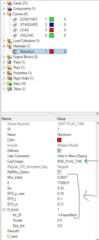
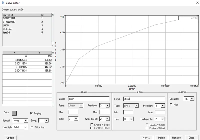
3.Create a curve from the curve card,so a curve editor box will open and click ‘new’ and name as ‘Law 36’ and proceed.
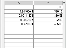
4.Create the curve using the x and y coordinate points and label X as Strain and Y as Stress and click ‘Update’.Assign the curve to the property in the Material card in ‘fct_ID’ region by selecting the ‘unspecified’.Name the material card as ‘Law 36’.
5.As a choice can assign the value of Tstop as 55ms in Cards>Engine Run and in Engine-Animation-DT,Tstart as 0 and Tfreq is 0.1.
6.In Analysis>Radioss,give the input file as (0000.rad) file and ‘tick’ include connectors which keeps in connected the surfaces and option as ‘-nt 4’ and click ‘Radioss’.
7.It runs the base simulation and gives the error file as (0001.out) file which consists of mass error,energy error,external work and at the end of file it should indicate ‘NORMAL TERMINATION’ which indicates successful simulation without any errors.
8.Now change the Client selector (ToolBar) from ‘Hypermesh’ to ‘HyperView’ to create the animation of crash.Upload the file (h3d) in ‘Load model and results’ of case 1 and ‘Apply’.Save the animation video.
9.Now change the Client selector from ‘Hyperview’ to ‘HyperGraph 2D’ where you need to plot the graphs which are given.
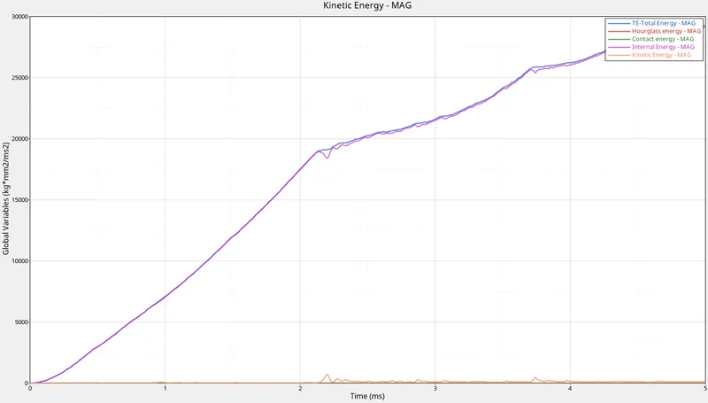
10.Plot the graphs for kinetic energy, internal energy, hourglass energy, contact energy, total energy of the simulations.
COMPARISON:
CASE 1 AND CASE 2:
CASE 1 CASE 2
CASE 1

 END OF CYCLE
CASE 2

 END OF CYCLE
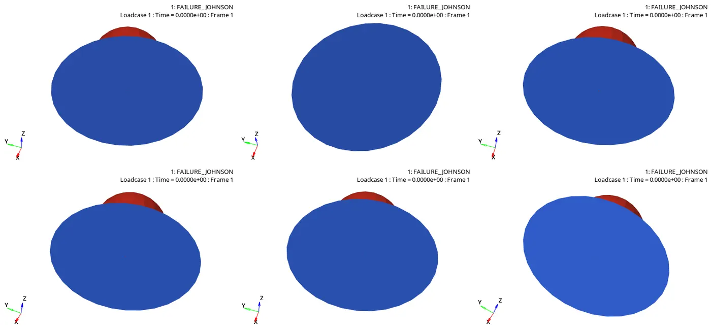
Comparision between case 1 and case 2:
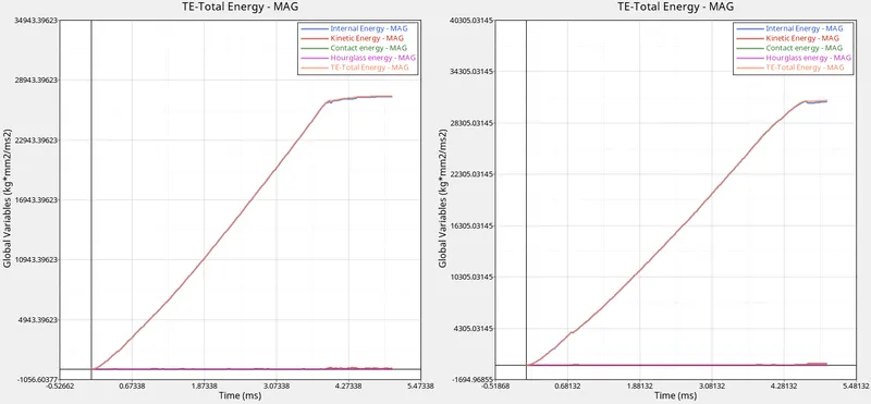
1.From the graphs and error files,we can observe that due to change in properties there is change in energies and time step.
2.By changing the Ifail_sh property from 2 to 1 in Failure card,the internal energy is decreasing in case 2 compared to case 1.
3.By changing the Dadv property in Failure card from 0 to 1,the time step is also decreasing as it advances the time step.
4.Due to change in properties like Ifail_sh,Dadv and ixfem,the kinetic energy is deviating at different time steps.
5.From the graphs,we can observe that hourglass and contact energy reamains constant due to Ishell=24 it stabilizes the hourglass energy.
CASE 3 AND CASE 5:
CASE 3 CASE 5
CASE 3

 END OF CYCLE
CASE 5

 END OF CYCLE
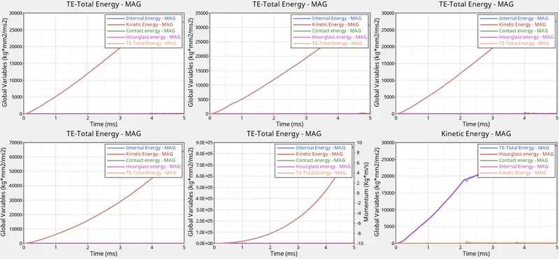
Observation between case 3 and case 5
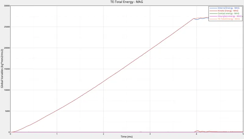
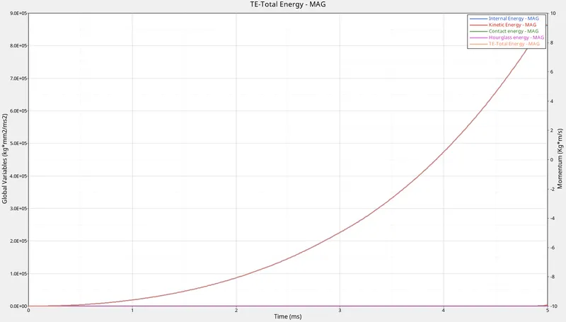
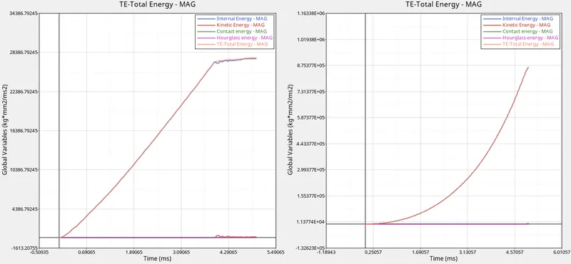
1.As case 3 is a Law 2 and case 5 is a Law 1,Law 2 is Elasto-Plastic Material and Law 1 is Elastic Materail.
2.In case 3,due to deleting the Failure card the time step decreases.
3.Due to delelting the failure card,the simulation wont take into consideration which were deleting and cracking.
4.The energy error was decreasing as which means deleting the failure card results in removing the advancement of error.
5.Total energy remains same as internal energy due to change in properties
6.In case 5,as we are converting the card image from Law 2 to Law 1,properties will get changed as Law 1 is Elastic Materail.
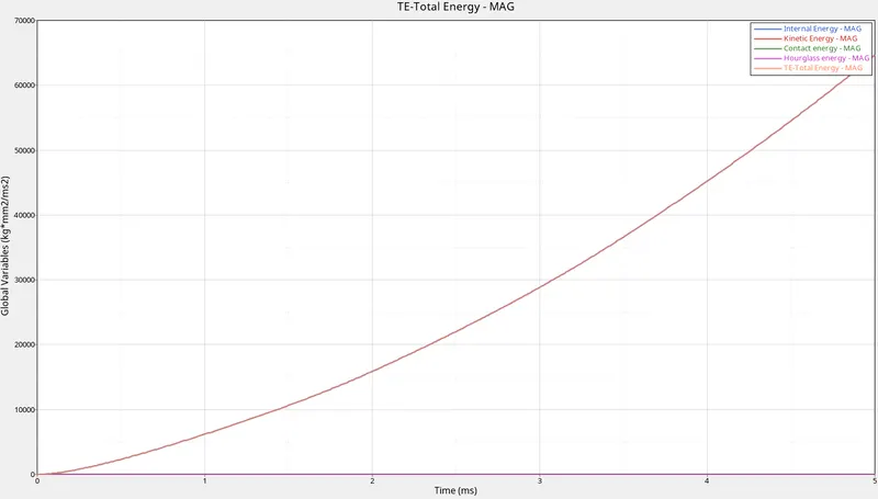
7.the internal energy graph will be exponentially increasing.
8.Due to property and materail change kinetic energy aiso decreasing.
9.This materail law is used to model purely eleastic material.
CASE 7:
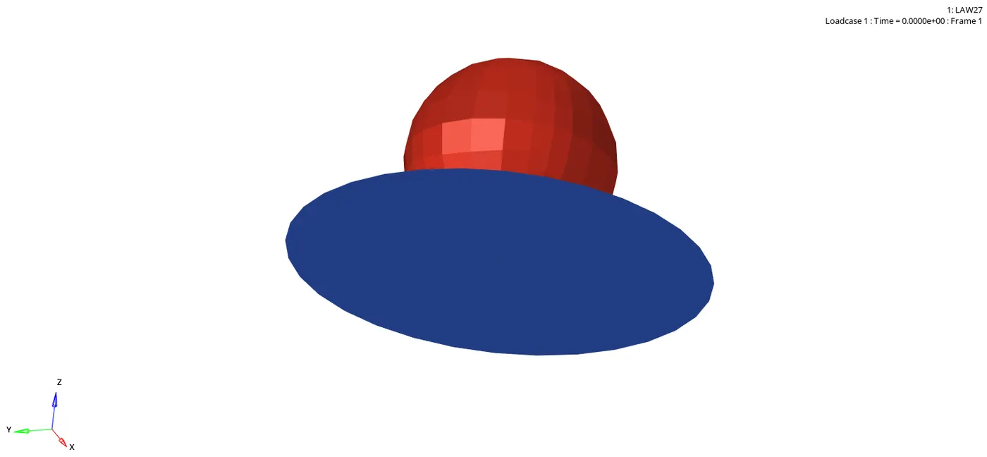
1.Import the LAW_27 Starter file(0000.rad) from Solver deck.
2.Assign the materail properties to the respective recommended properties.
3.As a choice can assign the value of Tstop as 55ms in Cards>Engine Run and in Engine-Animation-DT,Tstart as 0 and Tfreq is 0.1.
4.In Analysis>Radioss,give the input file as (0000.rad) file and ‘tick’ include connectors which keeps in connected the surfaces and option as ‘-nt 4’ and click ‘Radioss’.
5.It runs the base simulation and gives the error file as (0001.out) file which consists of mass error,energy error,external work and at the end of file it should indicate ‘NORMAL TERMINATION’ which indicates successful simulation without any errors.
6.Now change the Client selector (ToolBar) from ‘Hypermesh’ to ‘HyperView’ to create the animation of crash.Upload the file (h3d) in ‘Load model and results’ of case 1 and ‘Apply’.Save the animation video.
7.Now change the Client selector from ‘Hyperview’ to ‘HyperGraph 2D’ where you need to plot the graphs which are given.
8.Plot the graphs for kinetic energy, internal energy, hourglass energy, contact energy, total energy of the simulations.


OBSERVATION:
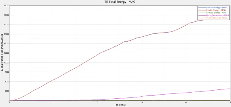
1.Due to Ishell=0 hourglass energy occurs.
2.Contact energy in constant.
3.This law is applicable for shells.
4.TIme step is reducing due to change in properties.
5.Total energy is increasing due to material change.
6.Failure and damage occur only in tension.
7.This law combines with Law 2 and brittle failure,causes damage before failure.
RESULT:
Completed the simulation and Plotted the graphs for internal energy,hourglass energy,Contact energy,Total energy and kinetic energy.
CONCLUSION:
Change in parameters in Properties(comparing case 1,2,3) getting elements deleted before the time step when compared to case 4 which exhibits elastic nature due to failure card.
As different laws exhibit different nature depends on the parameters of Properties.