Week - 9 Material Modeling from Raw Data

#10 // Week - 9 Material Modeling from Raw Data.

Aim: To perform the simulation and validate the curve as shown in the figure (Raw data) with the simulation post-processing curve.

Objective:

• Using the given video link, extract the data from the figure, and used it for validation.
• Create a material model for the Dogbone specimen using the diagram of the true stress-strain curve (graphite iron).
• From the above condition simulate and validate the material model by performing a tensile test on a Dogbone specimen.

Introduction:

It is very important to convert the material data into a material law that the solver can understand. To model the linear behavior of a material we just need the density, Young’s modulus, and Poisson ratio.LS Dyna consists of the following materials cards as shown below:

• Elastic

> Linear: Isotropic (MAT00)

> Non-Linear: Hyperelastic(MAT*077): Orthod aniso trophic: Their properties change with direction.

• Elastic -Plastic: These can be rate-dependent or rate independent.

The following laws are used:

> MAT003: PLASTIC KINEMATIC:

> MAT0012: Isotropic Elastic Plastic:

> MAT0015: Mat_Johnson_Cook: This considers the thermal and damage effects.

> MAT098: Simplified_Johnson_Cook: This does not consider the thermal and damaging effects.

The following material cards are used the most to model metals:

Mat_024, Mat_18 and Mat_098

• For a Rigid material we can use Mat_20

Elastic materials can be defined as shown below:

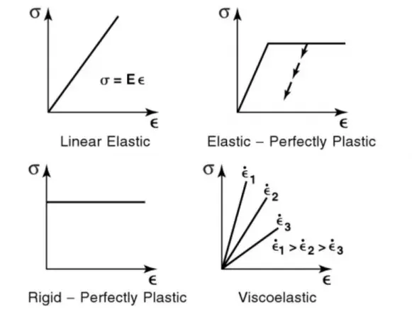
Strain rate is the rate of deformation caused by strain in a material within a corresponding time. This gauges the rate at which distances of materials change within a respective period of time.

To input the model, the material we have to convert the engineering stress-strain into true stress and strain by the following formula:

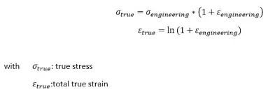
Once we get the true stress-strain curve, we convert it into a plastic strain curve and feed this data into the material modeling.

Now we will discuss hyperelastic material:

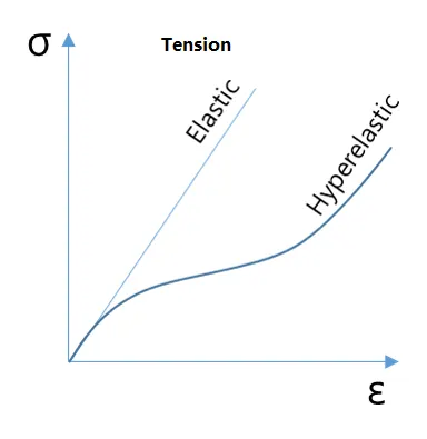
Hyperelastic material models are regularly used to represent the large deformation behavior of materials with FEA. They are commonly used to model the mechanical behaviors of unfilled/filled elastomers. In addition to elastomers, hyperelastic material models are also used to approximate the material behavior of biological tissues, polymeric foams, etc.

Linearly elastic materials are described through two material constants (like Young’s modulus and Poisson ratio). In contrast, hyperelastic materials are described through a strain-energy density function. The strain-energy density can be used to derive a nonlinear constitutive model (i.e., stresses as a function of large strain deformation measures like deformation gradient or Cauchy-Green tensors, etc.). There are several models proposed in the literature such as the Neo-Hookean, Mooney-Rivlin, and Signorini models,

Theory:

Stress-Strain

For the material, the engineering stress–strain curve plots the correlation between stress and strain. It is obtained by gradually applying a load to a test coupon and measuring the deformation, from which the stress and strain can be determined e.g. By tensile testing. These curves provide the material properties, such as Young’s modulus, yield strength, and ultimate tensile strength.

• The term Engineering stress is the applied load divided by the original cross-sectional area.
• The term True stress is the applied load divided by the actual cross-sectional area (changing area with respect to time).

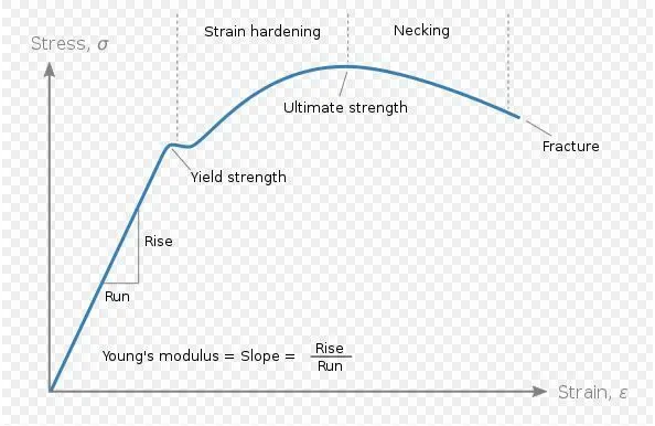
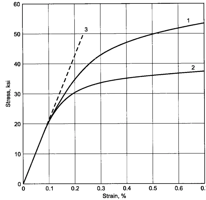
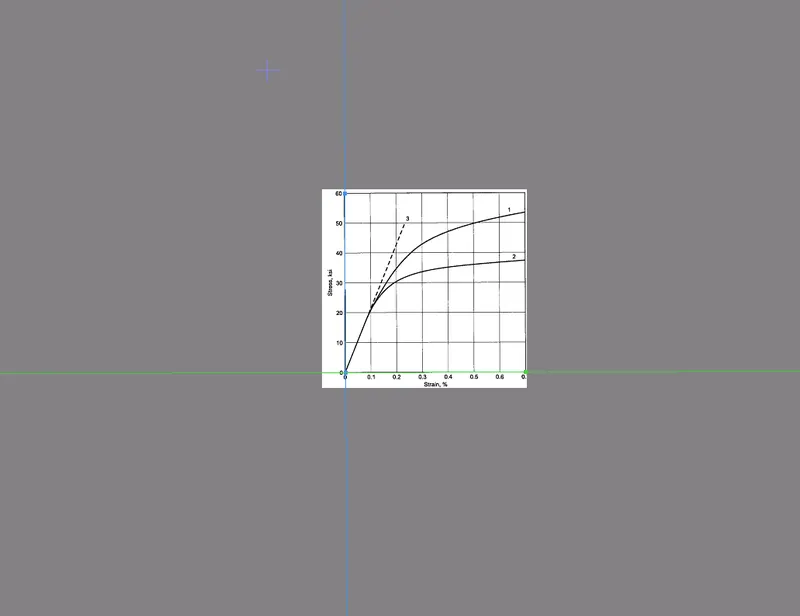
• The above image depicts the stress-strain curve from the graphite iron casting. The two curves with different material structures have been shown in the figure.
• This acknowledgment should be occupied from either MAT_024(Piecewise linear plasticity) or MAT_018(Power law of plasticity) material model according to the problem statement.

Procedure:

Data Extraction & Graph calculation ->

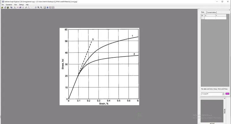
1. First import the stress and strain data from the stress-strain curve by using a data digitizer.
2. Import the Stress-strain curve image in the data digitizer as shown below.

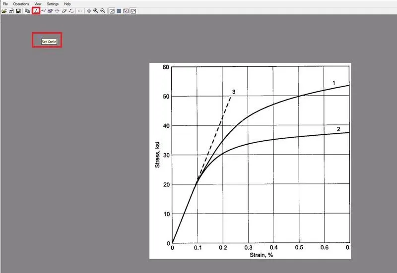
3. Next click on the set scale it shows the set Xmin, where we want to Xmin select by using the cursor and entering the value as 0 as shown below.

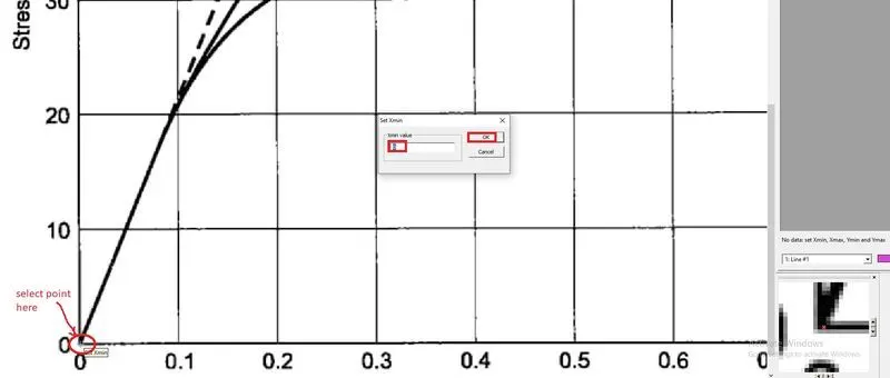
4. Click on ok next shows the set Xmax select X-axis maximum point and give the value 0.7.

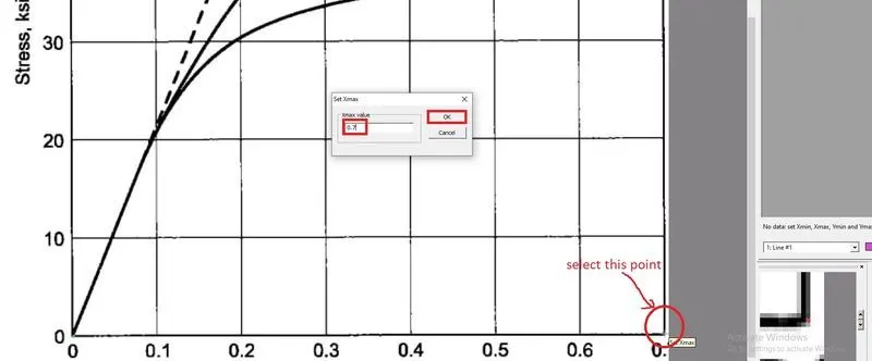
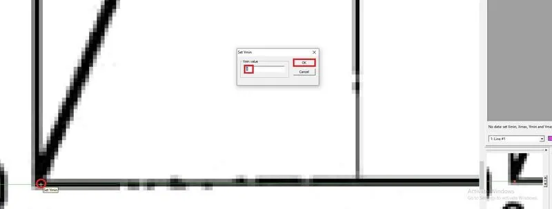
5. Next it is asking set Ymin to select the Ymin point and give the value is 0.
6. Next ask the set Ymax to select the maximum point in Y-axis and give the value 60.

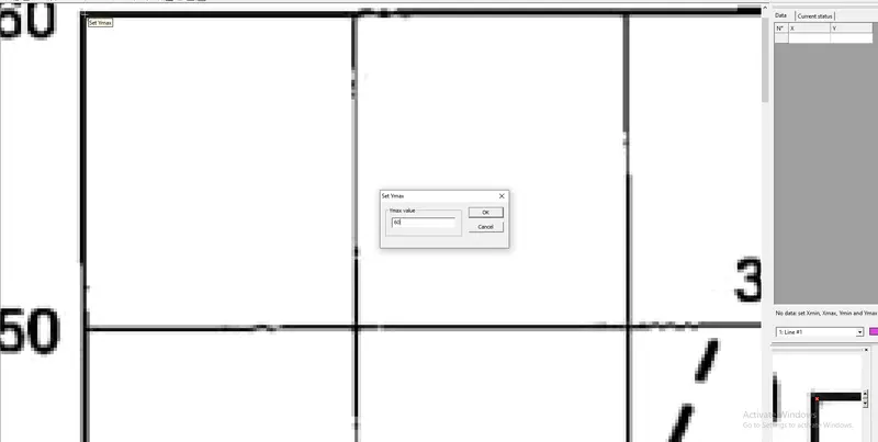
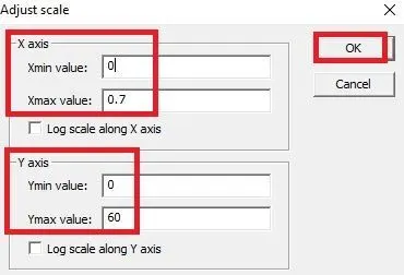
7. Next shows the dialogue box and see the minimum and maximum values and click ok as shown below.

8. It shows X-axis is a green line and Y-axis is a blue line as shown below.

9. Next select the point capture mode and pick the points randomly along the curve path 2 as shown below.

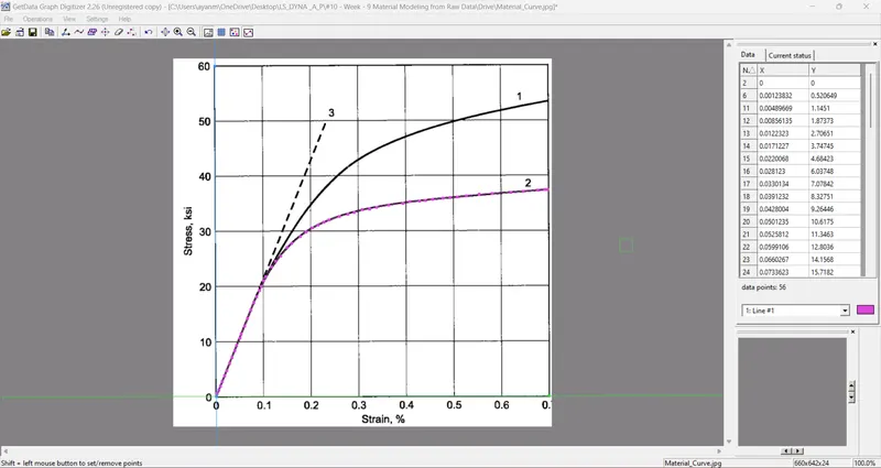
10. Next Export the data to Excel format and save the data.
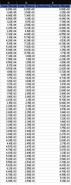
11. Next open the file in Excel it shows the stress and strain values as shown below.

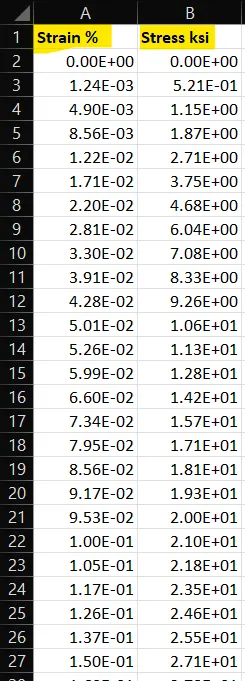
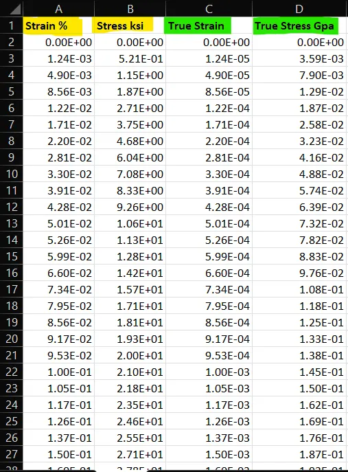
12. Here strain in percentage and stress in kilo pound-force per square inch (KSI) so convert both values as shown below.

Strain % = 10^-2

Stress 1 ksi =0.00689476 Gpa

so, we have multiplied the values for strain = strain % ×10^-2

For stress = stress (ksi) × 0.00689476

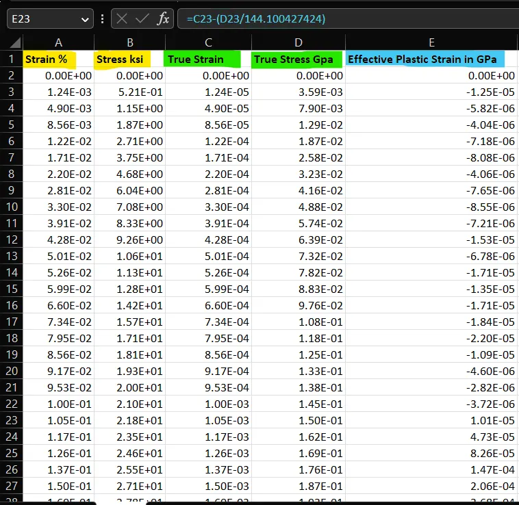
13. Next find the effective plastic strain as shown below.

Effective Plastic Strain = True strain - (True stress / Young's Modulus)

Here,

True stress = Stress

True strain = Strain

Young's Modulus E =20.9E+06 pound-force per square inch (PSI)

change the units of Young's modulus PSI to Gpa as shown below.

20.9E+06 PSI = 144.100427424 Gpa.

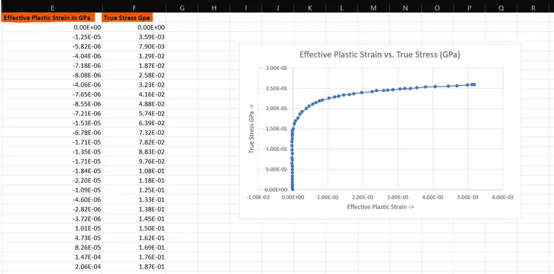
14. Plot the graph Effective stress vs Effective plastic strain. Here effective stress is nothing but True stress.

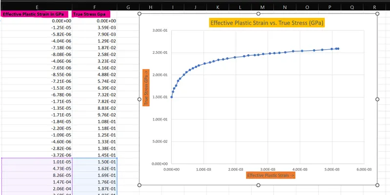
15. In the above image up to 0.15 it is linear above 0.15 it is non-linear so we have taken the values above 0.15 as shown below.

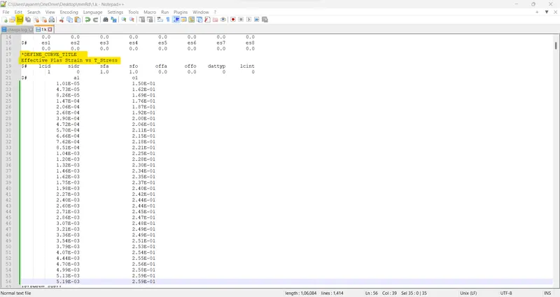
16. Next open the keyword file in the notepad and assign the above values for the Mat_curve as shown below.

17. Next save the file and open it in the LS-Pre post check the mat curve as shown below.

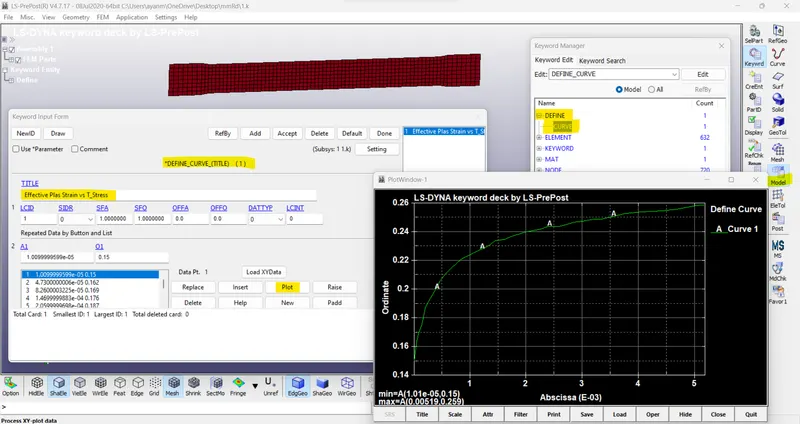
//Note- First create a mat_card & Define a curve in LS-Dyna & save it, Then open the file in Notepad++ & put Effective Plastic Strain, and True Stress values there. / use 'alt + select rows', and 'tab/space' to the appropriate position in Notepad. In the end, save it & open it in LS-Dyna.//

18. Next create the material 024 and section shell as shown below.

Material:

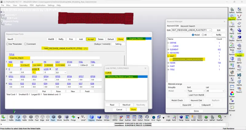
• The material card chosen is MAT_24_PIECEWISE_LINEAR_PLASTICITY to define the behavior of an elastoplastic material with an arbitrary stress-strain curve
• The values of Density and Poisson's ratio are taken as generic values. The young’s modulus = 20.9E+06 psi --> 144.1004 GPa, yield stress value from graph = 0.151 GPa
• The plastic behavior of the material is defined using the LCSS curve option. The curve is defined by inputting the values of effective plastic strain and effective stress (true stress)
  To define the LCSS curve the stress values beyond the yield stress values are considered.

Section:

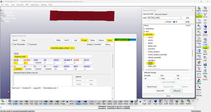
• The section property of the dogbone specimen is assigned as a shell element with 1mm thickness along with ELFORM=2 (Belytschko-Tsay)

19. Part:

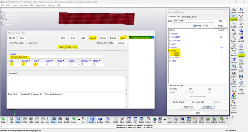
• The material and section are assigned to their respective part ID.

20. Next create the Boundary Conditions as shown below.

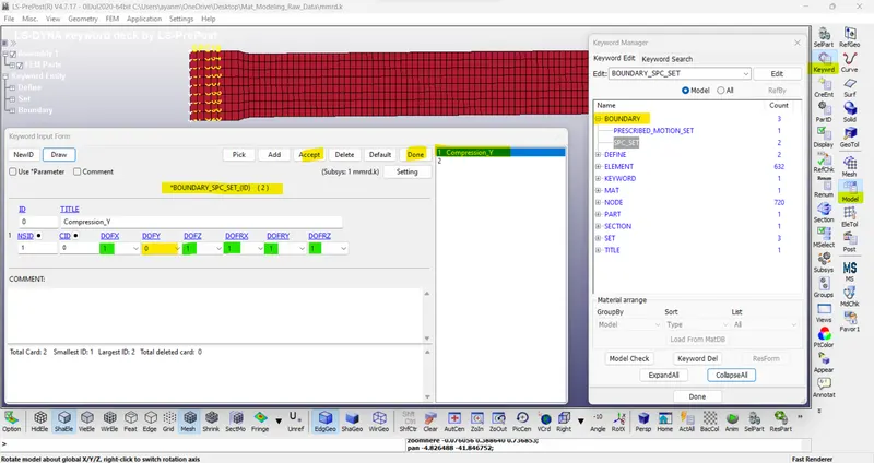
SPC set:

• The nodes at the fixed end are constrained in the X and Z direction, the Y direction is not constrained because of lateral compression during the tensile test.

SPC constraint y:

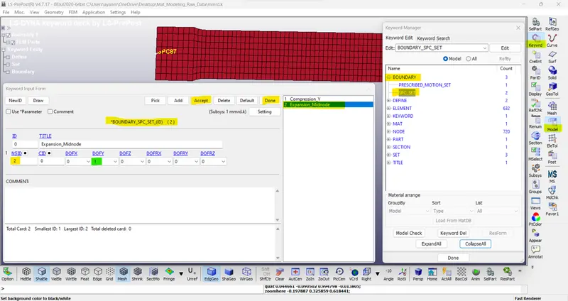
• The nodes in the middle are constrained in the Y direction since the neutral axis passes through the middle of the specimen in the X direction.

Prescribed Motion set:

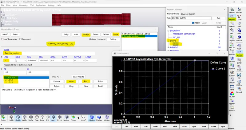
21. Create the curve for displacement as shown below.

22. Assign the displacement curve to the Prescribed Motion set as shown below.

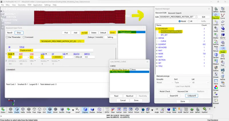
• The nodes pulling at one end are assigned with a boundary-prescribed motion in ‘-X’ direction using VAD displacement with a load curve of -1.0 m/s.

23. Control Cards:

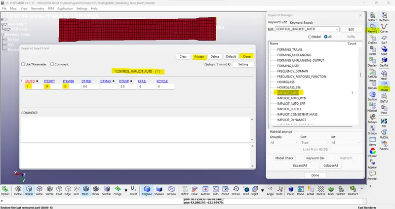
• To activate implicit analysis and define associated control parameters. The following keyword is required for all implicit analyses.

Implicit_Auto ->

IAUTO: set to 1 which automatically adjusts the timestep size
ITEOPT: optimizes the operation count step 11
ITEWIN: is the iteration window 5
DTMIN: Minimum allowable time step size 0
DTMAX: Maximum allowable time step size 0

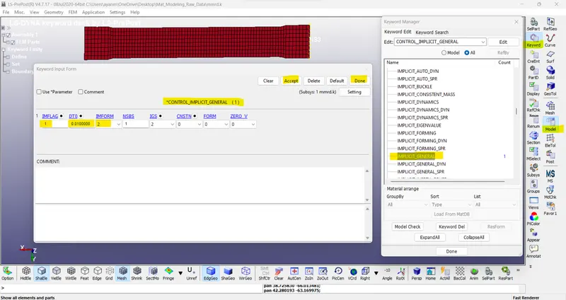
Implicit_General ->

IMFLAG: Implicit/Explicit analysis type flag: 1- Implicit analysis

DT0: Initial time step size for implicit analysis: 0.010000

IMFORM: Element formulation flag for seamless spring back: 2 retain original element formulation (default)

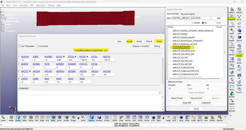
Implicit_solution ->

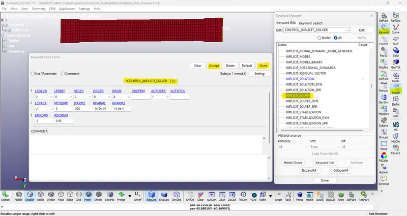
Implicit_solver ->

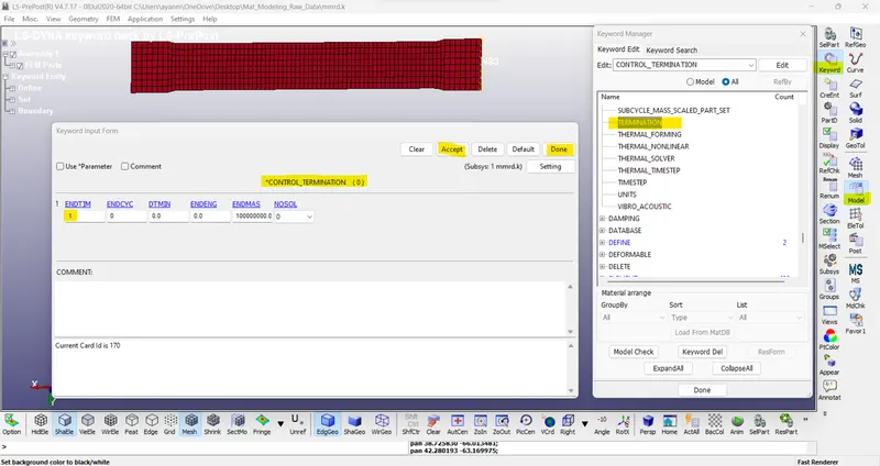
Termination:

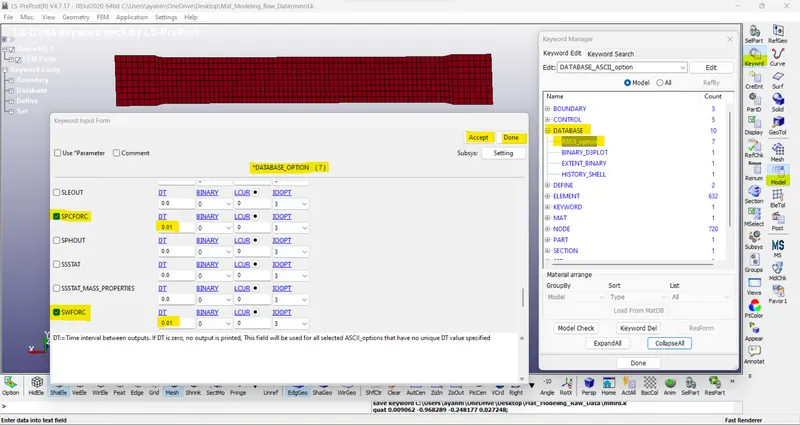
24. Create Database cards as shown below.

ASCII_options give the outputs ELOUT, GLSTAT, MATSUM, NODOUT, RCFORC, SWFORC, and SPCFORCE.

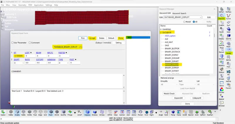
Binary_D3plot ->

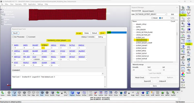
Extent Binary ->

History Shell ->

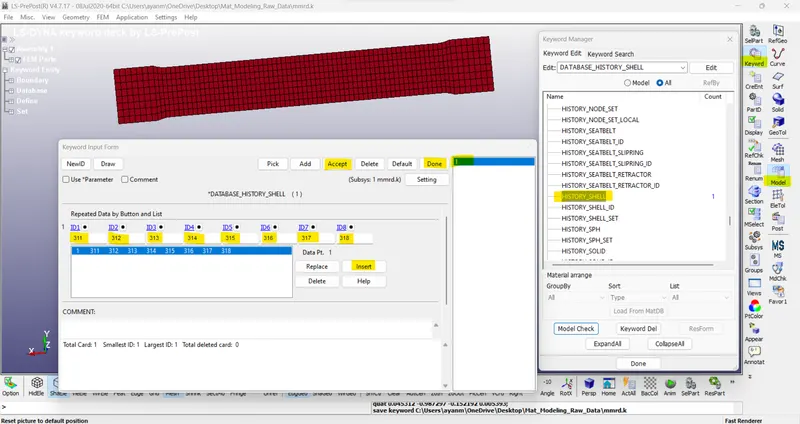
25. Save the keyword file and run the simulation in LS-Run.

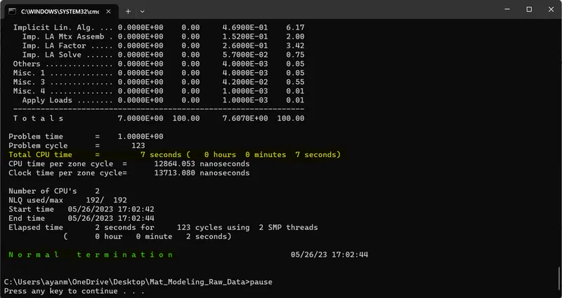
Post-Processing ->

Results-

/ CONTOUR PLOTS OF VON MISES STRESS -

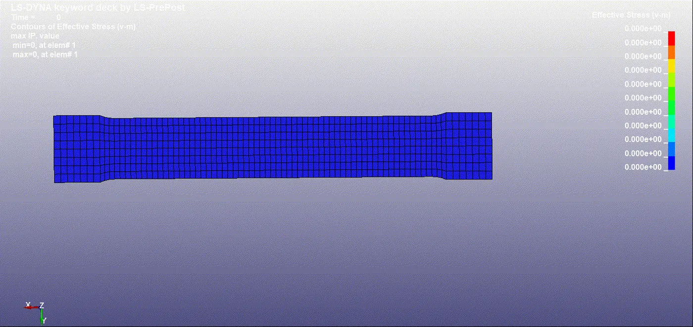
/ CONTOUR PLOTS FOR EFFECTIVE PLASTIC STRAIN -

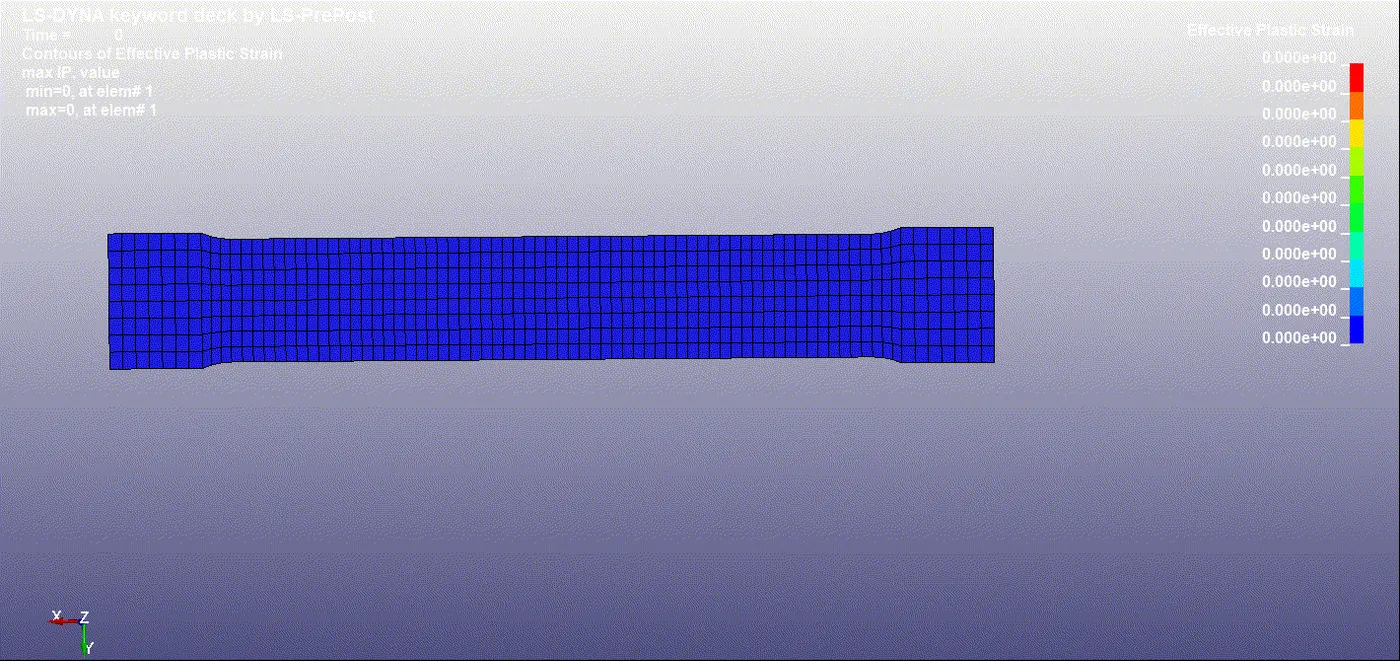
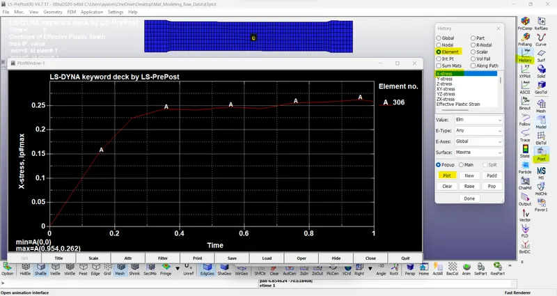
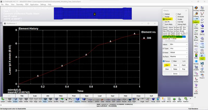
Stress vs Strain -

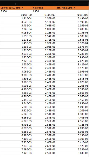
• The true stress vs true strain plot obtained from the simulation of the tensile test on the dogbone specimen is as shown in the image given below which resembles the given true stress vs true strain plot.

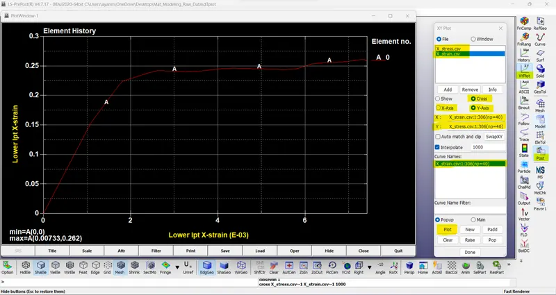
// Cross-plot True Stress vs True Strain -

Validation

• The Material-defined stress-strain data and simulated stress-strain data are distinguished by the elastic part as linear
  The linear elastic part is calculated directly through the given Young’s modulus and the yielding portion starts at the defined point in the hardening curve.

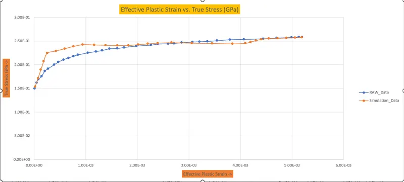
• There is an exact correlation between the experimental data and the given raw data.
• Due to some non-linearities, there could be some deviation that is tolerable.

/ Raw Data -> / Simulation Data ->

Conclusion:

The stress-strain data is extracted and validated from the image using a Data digitizer by MAT_024(Piecewise linear plasticity) which captures the actual stress-strain behavior similarly.
Few variations in the simulation data lead to a lack of information data from Density and Poisson’s ratio for the raw data.