Assignment 5-RADIOSS Interfaces & Study of Effect of Notches Challenge

#14 // Assignment 5- RADIOSS Interfaces & Study of Effect of Notches Challenge.

AIM:

CASE_A ->

• Create the 2D mesh for bumper assembly.(mesh size should be 6mm.)

CASE_B ->

• Create different type of interfaces, assign recommended values to the interfaces and compare the base simulation setup results with different kinematic condition simulation results.

OBJECTIVES:

• Create the mesh for bumper assembly,mesh size should be 6mm.

1. Run the crash tube model as it is.
2. Change the Inacti=6 and run.
3. Create the type 11 contact and run.
4. Remove both notches and remove boundary condition on rigid body node then run.
5. Create a new notch in the middle, select the whole section and run.
6. Create a new notch with nodes only from opposing 2 faces and run.

// Note:

• The widely used unit system in industries to develop a deck in the hypercrash is: KN, mm, ms, Kg.
• When a file is exported from the Radioss (Hypercrash), It will create another new 0000.rad file. And it will store the previous 0000.rad file as a backup file (as 0000.rad.bak). And also, it will create a M00 file (Which stores the data of tree & weld data).
• If that M00 file is deleted, in hypercrash we don't get the connection in our list of trees. But they will be represented as a type 2 contact interfaces.
• In hyper crash, the engine cards are represented as control cards. And the data history file is seen in T01 file.

THEORY:

• Interfaces (or) contact modelling:

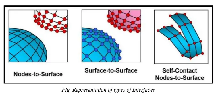
The interfaces are defined as a model how the parts interact, when they come into contact with each other. While discussing the interfaces, there are four types of interfaces widely used. They are:

1. Interface penalty method
2. Type 7, Variable stiffness, Node to surface contact
3. Type 11, Variable stiffness, edge to edge contact
4. Type 24, Linear stiffness, node to surface & surface to surface contact

Other type is Type 19, which is the combination of both type 7 & type 11.

Penalty method:

This method treats the behaviour between the slave nodes & master segments(surfaces) as springs that generate the resistive forces as a function of penetration, as shown in below figure.

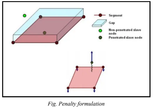
Time step is inversly proportional to the stiffness.

There are two types of time steps. They are:

• Nodal time step.
• Kinematic time step.

But the simulation is governed by the "Kinematic time step".

Type 7 ->

• This contact is used for node to surface contact.
• It can simulate all types of impact between a set of nodes and a master surface.
• It is non-oriented & slave nodes can belong to the master surface. Hence, the auto-impact is possible (can also be a self-contact).
• In this method, the penalty method with variable stiffness can also be used.
• Resistive forces are applied to keep the slave nodes out of the contact gap.
• Stiffness is non-linear.
• Contact gap can be constant or variable.

Contact gap: It's a gap between the slave nodes & master segment, which indicates when a slave enters in to that gap, which makes the resistive force come in to picture.

The resistive force vs penetration curve which is non-linear for the type 7 contact appears as shown in the below figure.

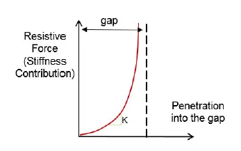
To have a stability, maintain the penetration lower level, which makes the stiffness less.

Important parameters in Type 7 ->

There are 7 parameters, which are important to be assigned at the time of creating the type 7 contact. They are:

Igap: Which determines the size of the gap is calculated.

Gapmin: To indicate the minimum gap for the activation of interface.

Inacti: Action to take, if initial penetration exists.

Istf: Affects how the stiffness of the stiffness is calculated.

Iform: To indicate the formulation of friction.

Stmin: To indicate, how much minimum stiffness to be used in the interface

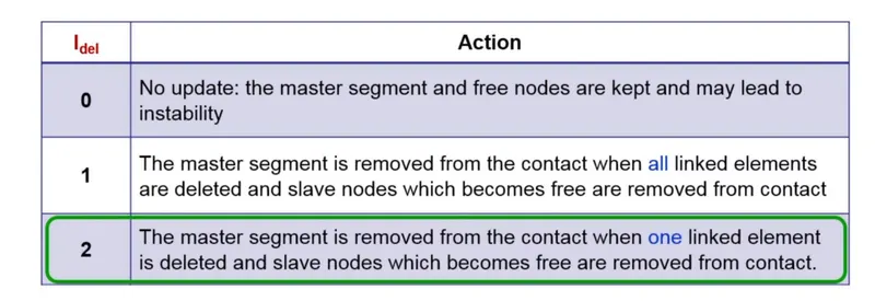
Idel: To indicate, what to do with the slave nodes & master segments if elements failed/deleted that they are attached to.

Igap:

Igap	Gap type	Description
0	Constant gap	The gap is defined by the Gap_min & is constant for all the contact. (Default)
1	Variable gap	Gap varies according to the characteristics of the impacted master surface & impacting slave node.
3	Variable gap	Variable gap with gap scale factor & mesh-size correction.

It depends on the Gap_min value (Recommended value for Gap_min is 0.5 mm).

Recommended value: 2 (or) 3.

Reason: Majorly, used is 3. Because, gap scale factor & mesh size correction is taken in to account. Because of adding gap scale factor, it puts a scale factor to the founded gap. In so many cases, there will be so many components with each other (i.e., By default the components will rest on each other). And if we don't want any reaction force to activate there. The Fscale gsp is going to relax the interface contacts by a bit. Which allows the slave node to reach up to the gap 0.8. Which reduces some calculations for solver.

Mesh-size correction: If the mesh size is big, then the nodes will be far away from each other. It is very likely, instead of nodes coming in to contact with the master segment, the edge of the slave node or element comes in to contact with the master. Because, the contact is not well defined. If the mise size correction factor, it can be overcome.

Limitation of Type 7: It will consider only the nodes as a slave nodes.

Inacti:

Before discussing about Inacti, the initial penetration should be understood.

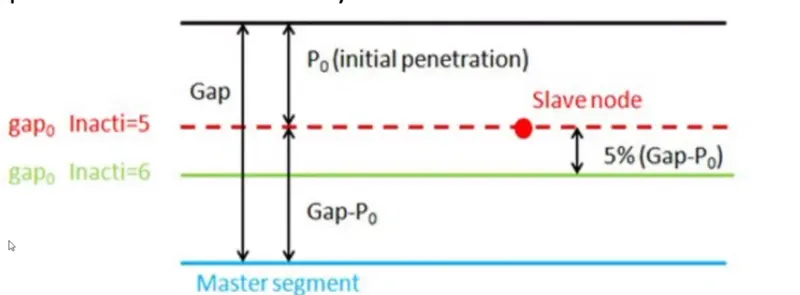
Initial penetration: Some nodes even pass behind or past to the master segment or element as shown in the below figure, which causes locking in simulations, leading to the computational failure.

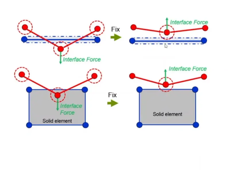
This can be overcome by using a fix algorithm. After using it would be like, which puts a load on simulation, which leads to the pushing force going on this node, which results to the energy error in the simulation. There are so many values, and the recommended is 6, as shown in the below figure.

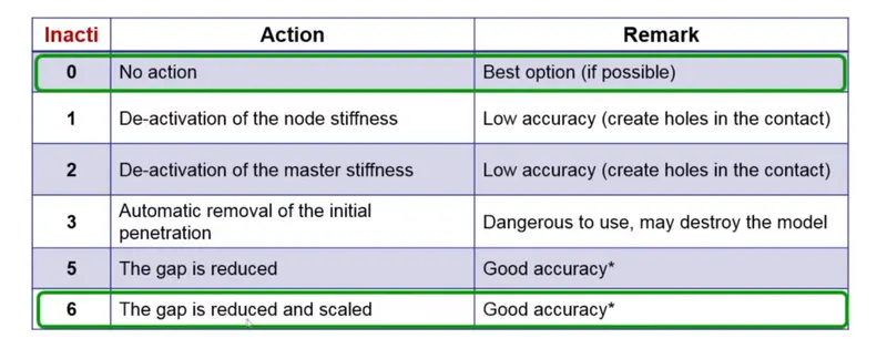
Reason: In case of going for value 5, it will scale down even further to as compared to case 5; the gap is reduced to P0 as shown in below figure. Because of that, In the case of vibrations at the slave side, the contact will get activated & deactivated. Which creates the problem. But where as in case of 6, it will scale down even further too, in such a way like less than (Gap-p0). Which in dictates the less gap when compared to (Gap-p0) of inacti 5. This leads a slave node to vibrate. Because of sound wave propagation through it, which reduces the contact calculations & increases the stability of simulation.

\

Istf:

The recommends value is 4. The reason is: Because of minimum stiffness, the resistive forces that are being applied on the slave node will be kept to minimum.

k = Max [stmin, min (stmax, Ko)]

where, Ko = min (Km, Ks); Km---> Stiffness of master segment, Ks---> Stiffness of slave nodes.

Example: If a soft component is coming in contact with a hard component, The soft component is going to absorb more resistive force & so that the stiffness of soft component should be considered. Because, the component is soft, its stiffness is less. The final value for contact stiffness, can be bounded by lower (Stmin) & Upper limits (Stmax).

Iform:

Iform means "sliding force computation". The recommended value is Iform: 2.

Reason: Because the, sliding forces are computed using the stiffness parameters of the parameters. But whereas in Iform: 1, the sliding forces are computed using the viscous parameters.

Idel:

The parameter "Idel" indicates the update for deleted elements due to failure. The recommended value is 2. The reason is shown in the below figure.

Finally, the recommended values for the parameters are: -

Igap = 2 (or) 3

Gapmin ≥">≥≥ 0.5 mm

Stmin = 1000 N/m (or) 1 KN/mm

Istf = 4

Inacti = 6

Idel = 2

Iform = 2

> Advantages & Disadvantages of Type 7 contact: -

Advantages:

• Physically correct representation
• High accuracy for describing the self-contact & buckling.
• Best used with shells to shells (or) solids to shells.

Disadvantages:

• Requires more stringent modelling practices.
• Does not tolerate intersections (Slave node passing master segment).
• Time step may reduce due to increasing interface stiffness.
• With respect to the methodology, it will not see the contact due to edges crossing each other at angles.

Type 11 contact:

• It is also known edge to edge contact. In the case of edge crossing, type 11 interface can be added to capture the physics correctly.
• It is defined by identifying the master & slave lines in terms of edges.
• It works similar to type 7 contact in terms of penalty formulation, gap definition, search method.
• Slaves will receive stresses & forces. And the object which is to be analysed is the "Slave".
• Coarser the mesh, stiffer the structure. Hence the master is typically meshed coarser. So that the slave doesn't penetrate in to the master. That's why the less deformable (or) highly stiffer structure is taken as master & less stiff as slave.

Note: Type 19 contact is the combination of both type 7 & type 11 contacts.

Skew:

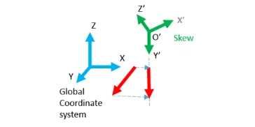
• Skew is one type of reference coordinate system which helps in defining local quantities with respect to the global coordinate system.
• Here the origin of the skew remains in a fixed position even if it is a fixed skew or moving skew.
• In a moving skew, the orientation of the node of interest is recomputed every time, with that of the origin coordinates of the skew.

Application: - The example is the study of intrusions in the car through skews. 2 nodes are created and fixed skews are assigned to it. There the travel of the node is computed from the global coordinates and it is presented in the local coordinates. The overall travel of the node is obtained.

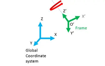
The skew is represented as shown in the below figure.

Frame:

• A frame is a type of reference coordinate system where the quantities defined follow its own origin.
• Here, unlike the moving skew, the moving frame is attached with the node which is selected as origin.
• It helps in Calculating the motion of the body relative to the frame defined.
• Frames are used only in notable options like imposed velocity, imposed displacement, TH/node etc. The frame is shown in the below figure.

> Tied contact/INTER/Type 2 ->

Definition: - It is defined as an interface that kinematically connects a set of slave nodes to a master surface. It can be used to connect coarse & fine meshes, Model spot welds, rivets etc.

• Slave literally follows whatever the master is importing over the slave.
• Slave nodes cannot have any motion by themselves. And if we put any constraints on the slave node except Type 2; it shows a pop-up like incompatible kinematic conditions.
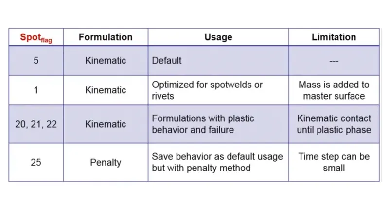
• It allows to use penalty method, which removes the potential incompatible kinematic conditions with the spot flag= 25. But in so many cases, Spot flag 25 is not recommended. Because, it will remove the errors automatically, which may lead to arise new problems. The different formulation for spot flag is shown in the below figure.

PROCEDURE:

CASE_A ->

• IMPORT:
• Given model is imported to Hyperworks using import model option.

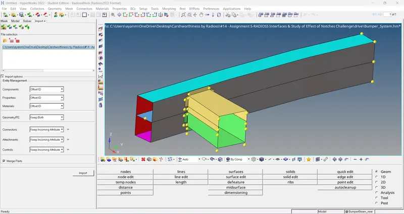
• The given model is viewed in topo mode to view the surface edges.

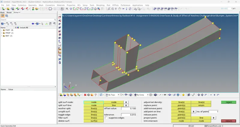
• Geometry Cleanup :

• Since the topo mode view shows the surface irregularities in the imported model, it should be cleared before meshing of the model.
• The geometric clean-up of the imported model is done using the following tools:
• For missing surfaces, filler surf option under quick edit tab is used
• For Disconnected edges, toggle edge option under quick edit tab is used.
• For Extend surf or surf to surf Trim, Surface edit option used.

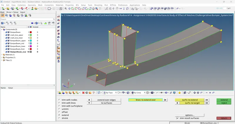
• MESHING:

• After the clean-up is finished and each simple surfaces are selected to obtain proper mesh.
• The meshing is done by using automesh tool under 2-D tab with elements size as 6mm and element type as mixed.
• The meshing of each component is done component wise.

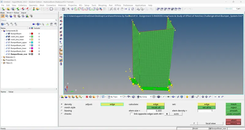
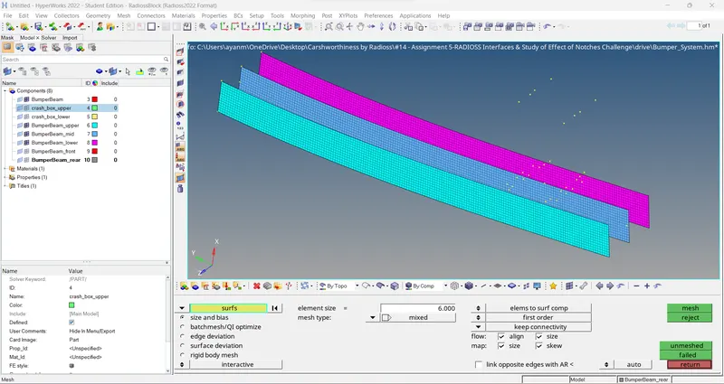
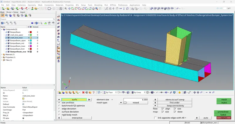
• Similarly meshing is progressed into adjacent surfaces to mesh the whole model and meshing is completed to obtain mesh as shown below:

CONCLUSION:

• Hence carried out geometry clean-up operation on the given model.
• Meshing performed on each component with elements size under the given quality criteria of 6mm.

CASE_B ->

OBJECTIVE:

To perform RADIOSS analysis on the given Crush Tube under given conditions and different notch locations.

Case 1:

Running simulation on the model as it is without changing any formulations.

IMPORT:

The given ".rad" file is imported as solver deck using import option.

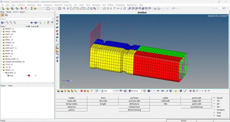
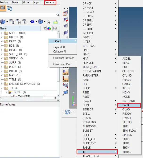
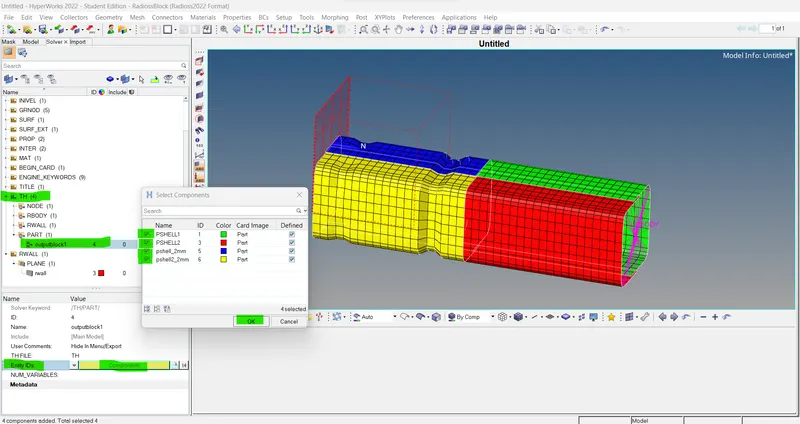
To create TH/Part, under solver browser, new TH -> PART option is selected and all the 4 components are selected.

Apart from that, we don't edit values in any parameters which come under the model browser. Perform the simulation as it is for all the cases.

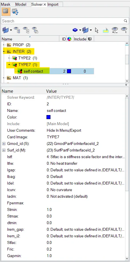
Important Interface parameters:

Igap : Determines how the size of the gap is calculated.

GAPmin : Minimum gap for activation of the interface.

Inacti : Action to takes if initial penetration exists.

Istf : Affects how the stiffness of the interface is calculated.

Iform : Friction formulation.

Stmin : Minimum stiffness to use in the interface.

Idel : Behaviour of slave and master segment if an element fails.

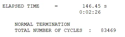
In the Radioss section, we can click 'save as' to save the file if it hasn't been saved yet. Care must be taken to include 'CASE_1_Crush_tube_0000.rad' in the file name since it's the starter file. After that, we can check the connectors option and input '-nt 4' in the options bar before clicking 'Radioss'. This starts the Radioss simulation, which will run for a few minutes.

Simulation is performed using RADIOSS option under analysis tab (Altair Compute Console Solver View), and the OUT file is viewed to check stability of the system.

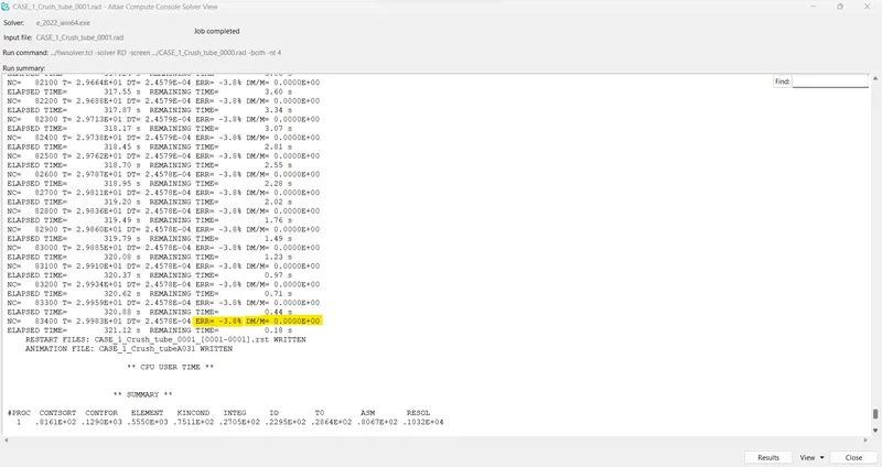
From the OUT file,

• energy error = 0% to -3.8%
• mass error = 0.00

Since the energy and mass error are within the acceptable range, the model is stable.

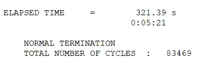
Now the time for simulation and number of cycles taken to complete the simulation is also noted from the OUT file.

Animation and Contour plot of the simulation is obtained under Hyperview using the h3d file saved in the directory.

It is observed from the animation that, the deformation of the tube under the action of force starts at the upper notch. on further loading, the upper notch gets fully bend, which on further loading, bending of the lower notch takes place. After both the notch region get bend, the upper part of the tube bends in a similar trend as that occurred in the lower part of the crush tube.

The crush tube gets fully deformed to a stage as shown below:

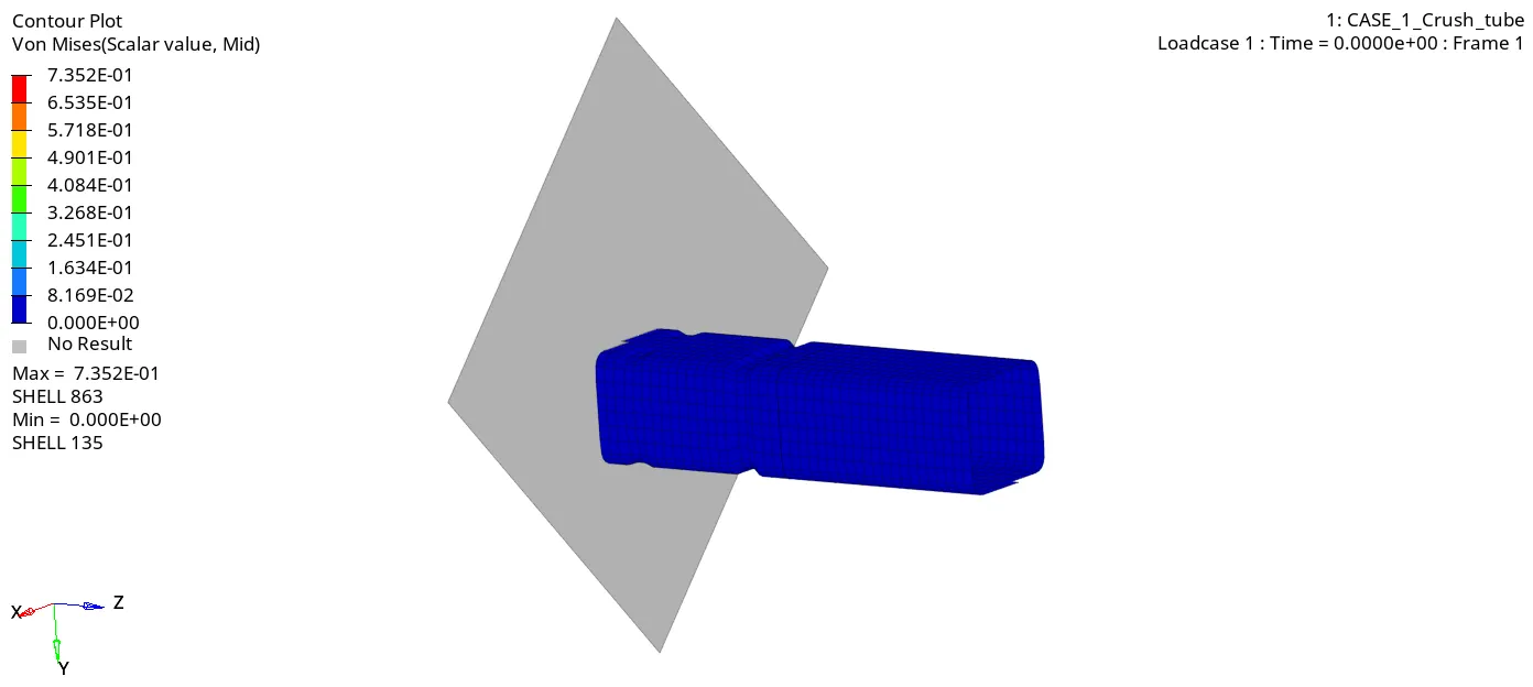
It is observed that, Von Mises stress values reaches a value upto a maimum of 7.352E-01 GPa.

> Plotting the energy curves using Hypergraph 2-D with the help of T01 File:

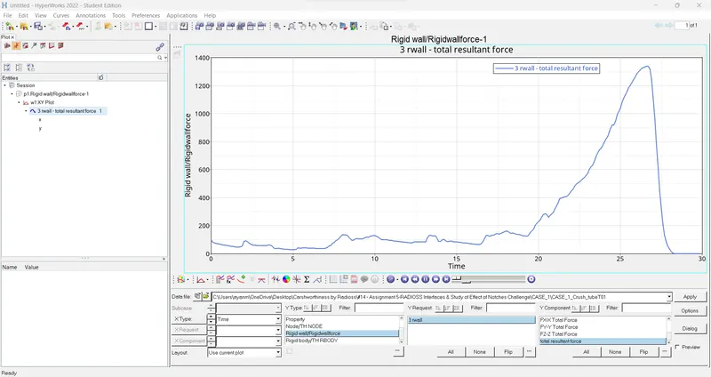
Resultant of the rigid wall forces is plotted and it can be observed that the rigid wall force rises with the deformation in the crush tube. After 20ms there is a steep rise in the force and finally reduces to zero when the tube is fully deformed and remains zero till end of the simulation.

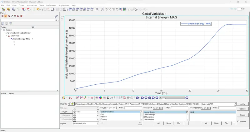
The internal energy of the system keeps rising till the tube is fully deformed and then remains roughly constant after 26ms till end of the simulation.

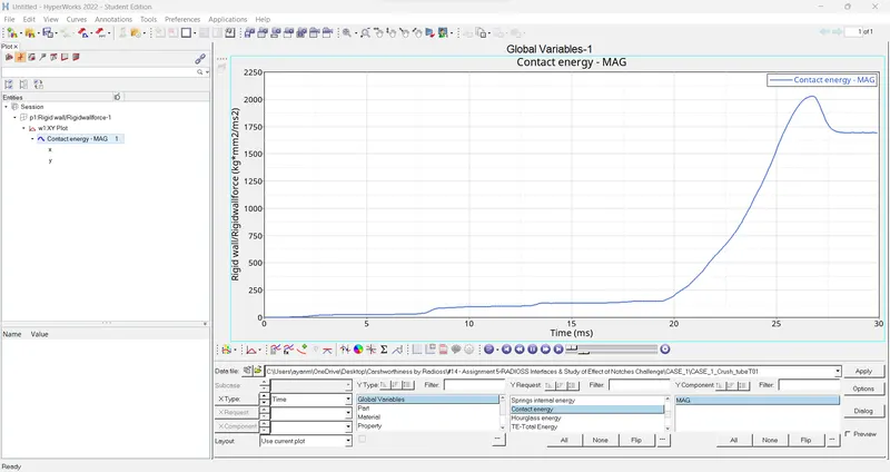
Contact energy of the system also rises due to deformation, and at a point rises with a steep slope till the tube is fully deformed, then reduces and remains constant till end of the simulation.

Case 2:

In this case, changed into 6 as an "Inacti" parameter and keep remaining things as it is.

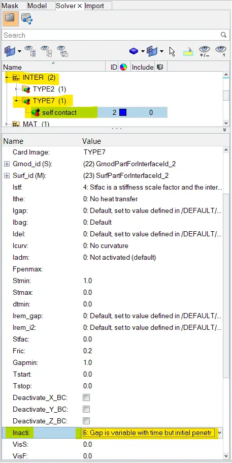
When we keep 6 to the "Inacti" parameter, it will remove the initial penetrations where possible. Elsewhere, reduce to less than 30% of the defined gap value and adjust the gap. In simple terms, the gap is reduced and scaled.

In order to change flag for inactivation of stiffness, Solver browser is opened under View > browsers > Hypermesh > Solver.

Under solver browser, INTER collector is expanded under which TYPE 7 is selected to modify the value of inacti.

Similarly, do the same thing as how we have done in the previous case. Select the "Radioss" sub-panel under the "Analysis" panel, save the file in the separate folder, and click the Radioss button to solve the problem by solver itself.

After calculating the model, a solver is generated different files such as the Starter listing file, Engine listing file, Animation files, Time history file and then restart file.

If the mass error has been falling in between -15 % to -5 %, that means the mass error is an acceptable thing. In this case, the error has been falling between -5 to 1 which means results are accurate and acceptable too.

A mass error has been zero from beginning to end, so it's an acceptable thing.

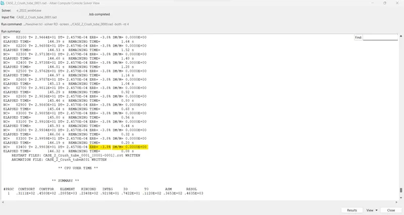
From the OUT file,

• energy error = 0% to -3.8%
• mass error = 0.00

Since the energy and mass error are within the acceptable range, the model is stable.

Now the time for simulation and number of cycles taken to complete the simulation is also noted from the OUT file.

After completion of solving, switch to "Hyperview" from the "HyperMesh" section.

Select the appropriate file in an "h3d" format and open the same file in the Hyperview interface.

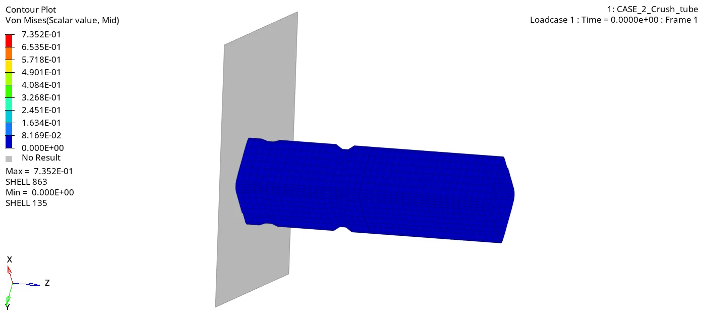
Contour plot for Von mises stress:

Stress generated around 7.352E-01 GPa for this case.

Seems to have the same behaviour as the previous simulation.

Switch to the "HyperGraph 2d" interface instead of the "Hyper View" interface for plotting the required one.

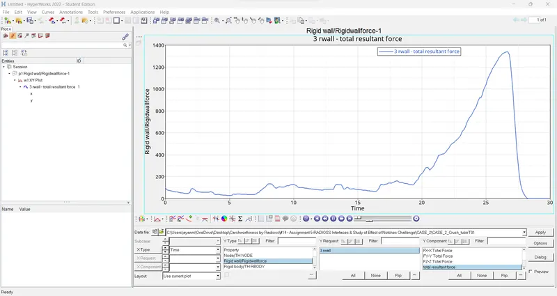
Rigid wall forces:

It will start from around 150, after 20 milliseconds it will start increased gradually up to 1400 afterwards rapidly return to zero at end of the simulation.

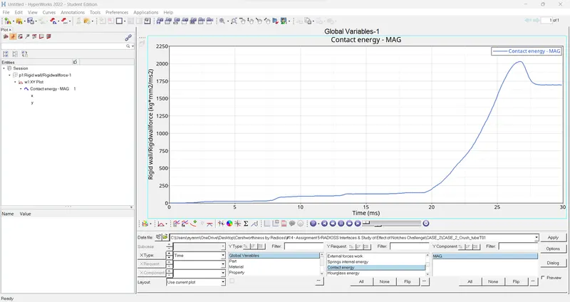
Contact energy:

Initially, it's goes increased slowly, after 20 ms it goes increased highly due to defined friction between them. At end of the few milliseconds, it maintained constant force due to happened the crushing.

Internal energy:

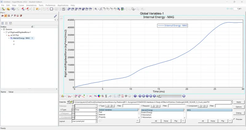
Initial energy starts from 0 and ends with around 42265 over the period of time. In the last few seconds, energy was maintained at a constant level because crushing has happened on the model.

Internal energy is higher than the previous case because keeping the "Inacti" parameter is 6.

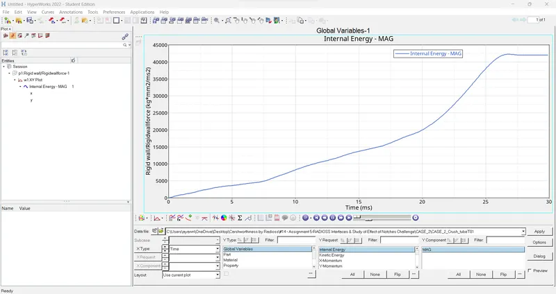
CASE 3:

In this case, use the same model, but change the contact interface to TYPE 11 instead of TYPE 7.

Change into "components" instead of "set" for the Slave & master line id and define the component.

Keep "4" as an "Istf" which means the solver will set the stiffness of the interface based on the softer of the master and solver.

Keep "3" as an "Igap" which means the gap varies according to the characteristics of the impacted master line and impacted slave line in addition to that a gap is taken into account the size of the elements.

Keep "2" as an "Idel" which means remove the slave nodes from contact because of element deletion.

Keep the value "1000" as a "Stmin" which means the solver will specify the minimum stiffness in the contact to avoid soft contact.

Keep "2" as an "Iform" which means sliding forces are computed using the stiffness of the interface.

Keep "6" as an "Inacti", a gap is reduced and scaled. And remaining parameters are kept as it is by default.

Keep "Gapmin" as an “0.5”.

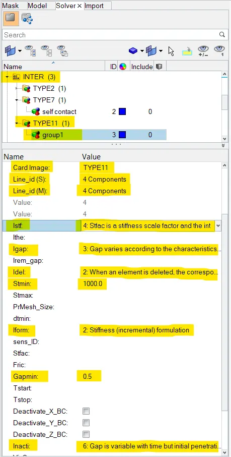
In this case, errors are falling within the acceptance range. An error is well control in this case as compared to the previous case.

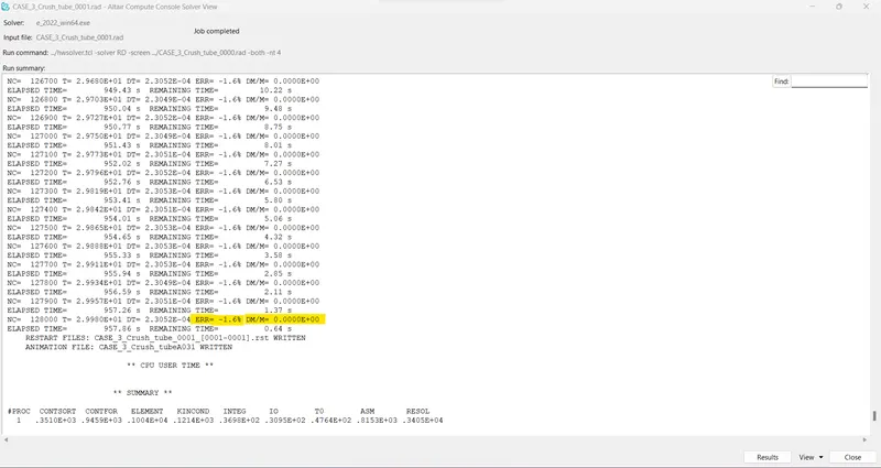
From the OUT file,

• energy error = 0% to -1.6%
• mass error = 0.00

Since the energy and mass error are within the acceptable range, the model is stable.

Now the time for simulation and number of cycles taken to complete the simulation is also noted from the OUT file.

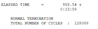
After completion of solving, switch to "Hyperview" from the "HyperMesh" section.

Select the appropriate file in an "h3d" format and open the same file in the Hyperview interface.

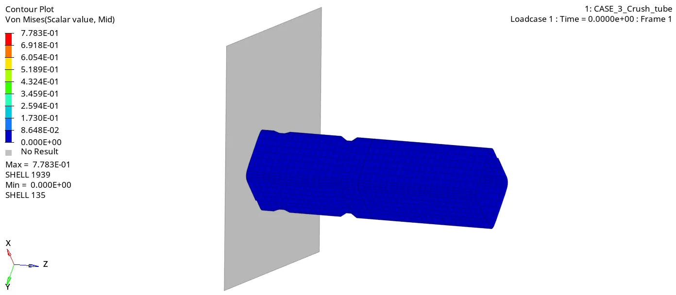
Contour plot for Von mises stress :

Stress generated up to 7.783E-01 GPa only from zero at the beginning.

A component starts deformation at the middle where the notch is located because there's less resistance strength on that area and also some stress flow interruption has happened.

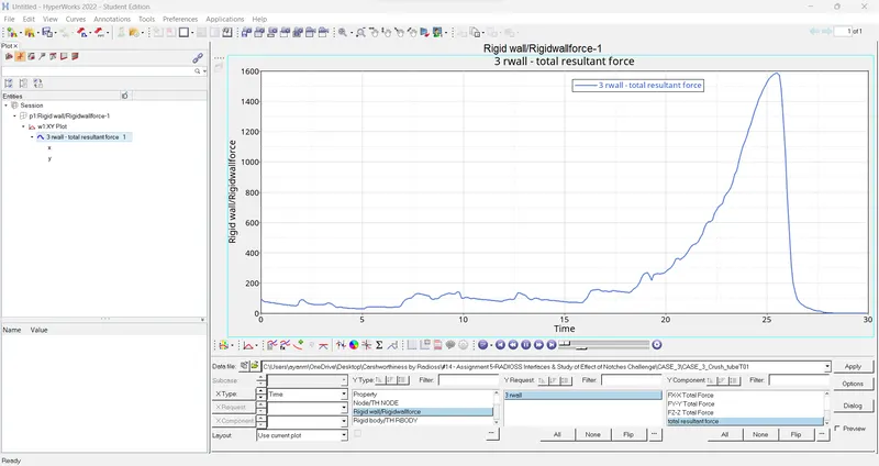
Rigid wall resultant forces:

A rigid wall force plot is followed by the same pattern as the previous one, but the maximum force has been reached 1600 kN.

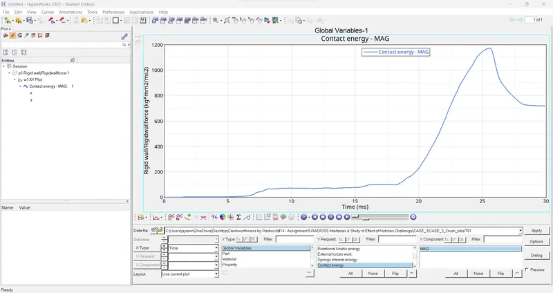
Contact energy:

Energy is not developed up to 7 ms, then it slightly increased & maintain constant force up to 19 ms. After 20 ms & up to 25 ms, it will linearly increase up to 1200.

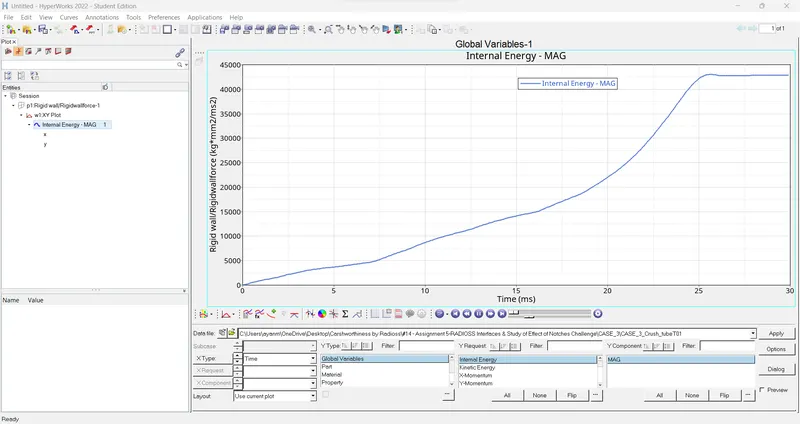
Internal energy:

Internal energy has started from Zero at the initial time and end up with around 45000 at the termination time.

CASE 4:

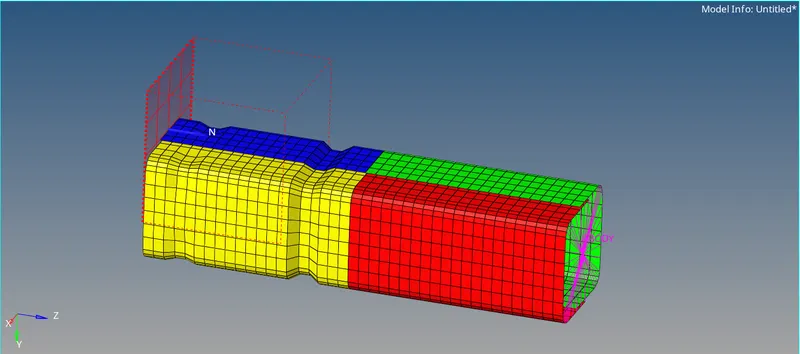
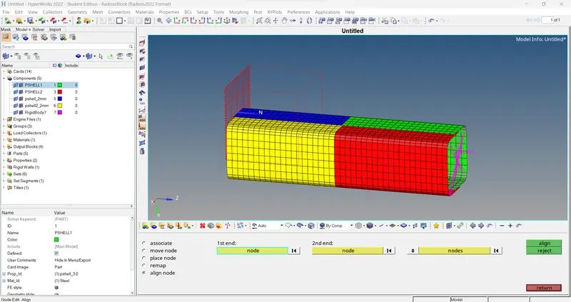
In this case, we have to remove the notched from the model using align node option which is available in HyperMesh. And also removed the boundary condition from the solver entity for this case.

> To remove the notches in the Tube, Node edit option under Geometry tab is used. Align node option is used to remove the notches on the tube profile.

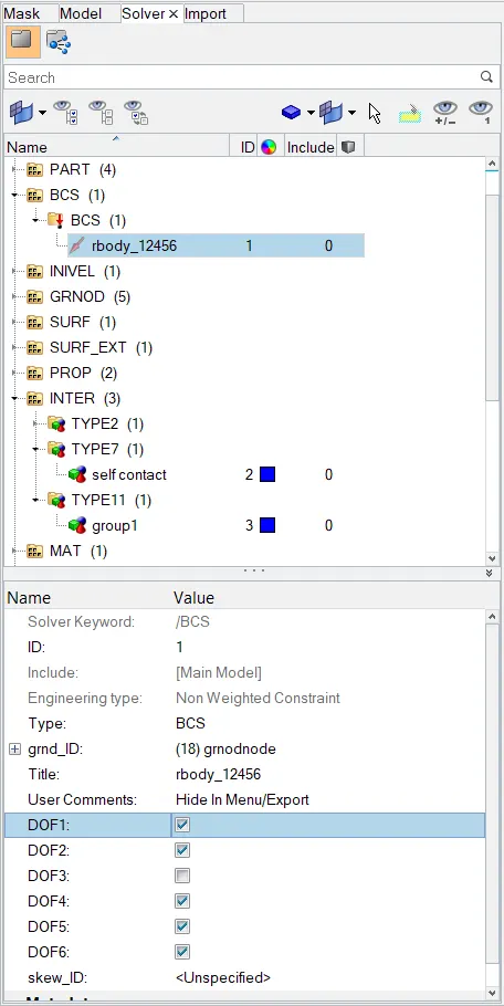
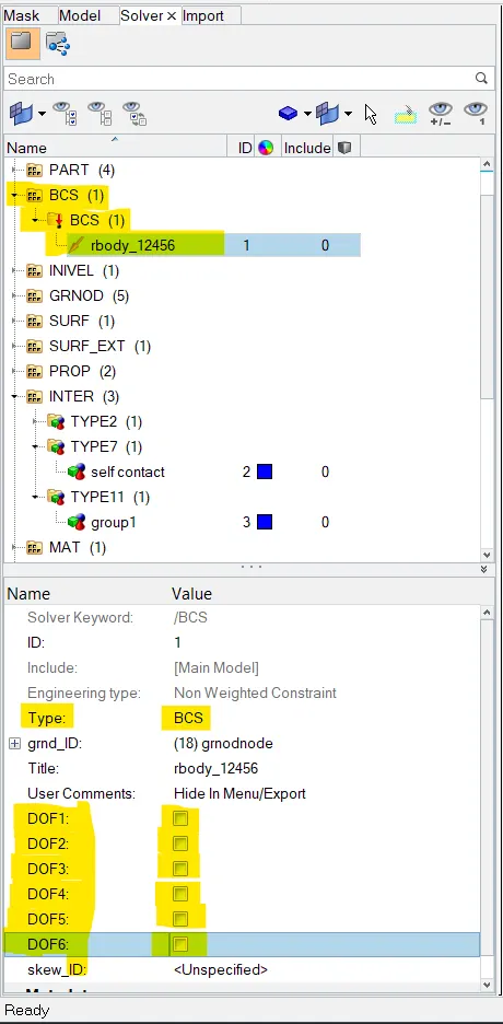
> To remove the rigid wall boundary condition, BCS collector under solver browser is viewed.

> All DOF conditions are removed to follow the given condition.

--->

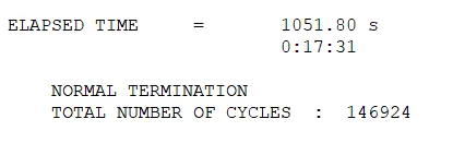
In this case, errors are falling within the acceptance range. An error is got as same as in the previous case, but it has taken more cycles to complete the solving.

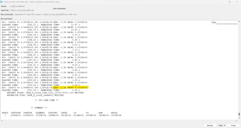
From the OUT file,

• energy error = 0% to -1.5%
• mass error = 0.00

Since the energy and mass error are within the acceptable range, the model is stable.

Now the time for simulation and number of cycles taken to complete the simulation is also noted from the OUT file.

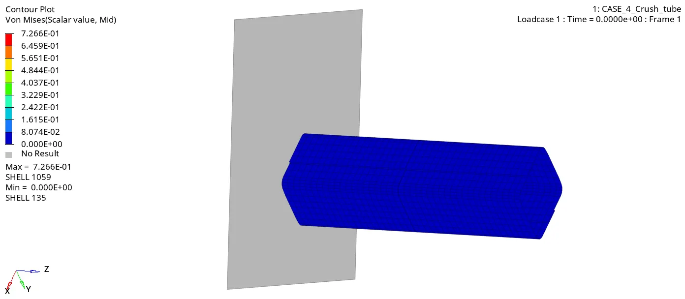
After completion of solving, switch to "Hyperview" from the "HyperMesh" section.

Select the appropriate file in an "h3d" format and open the same file in the Hyperview interface.

Contour plot for Von mises stress:

Stress generated up to 7.266E-01 GPa only from 0.

A component has been started deformation on the bottom because since we are removed the notch from the model.

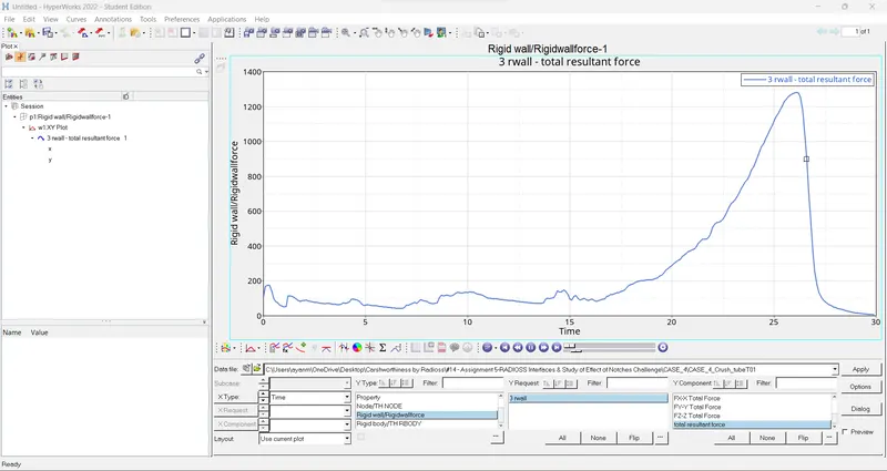
Rigid wall resultant force:

A Rigid wall force plot doesn't vary with & without notches on the component. Still, it has been followed by the same pattern and maximum force.

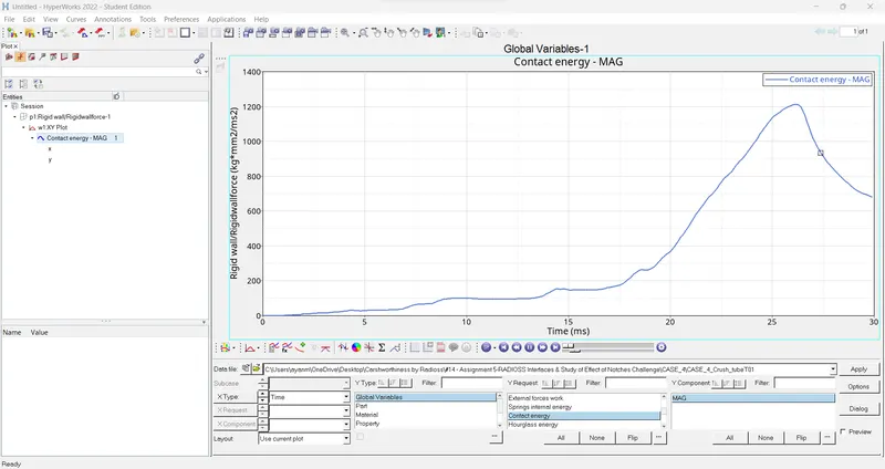
Contact energy:

Contact energy is not varied with & without a notch on the model.

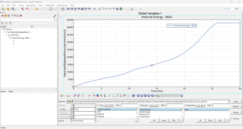
Internal energy:

Internal energy is not varied with & without a notch on the model.

CASE 5:

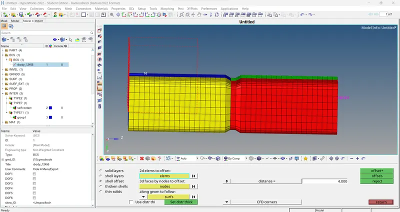
In this case, keep the middle notch only for solving as below.

To create the notch in the middle, Element offset option under 2D is used.

Go to 2D > elem offset > shell offset > 2D elems to offset > select 1 layer of elements > put distance (as per around half of average node distance) > offset+/- (as per needed)

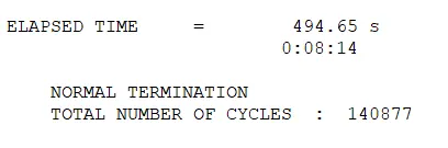
It took around the same number of the cycle as the previous one. Errors also become within the acceptable value range.

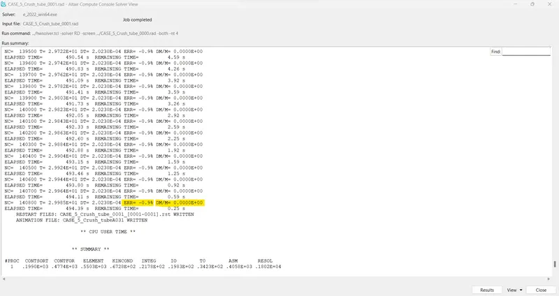
From the OUT file,

• energy error = 0% to - 0.9%
• mass error = 0.00

Since the energy and mass error are within the acceptable range, the model is stable.

Now the time for simulation and number of cycles taken to complete the simulation is also noted from the OUT file.

After completion of solving, switch to "Hyperview" from the "HyperMesh" section.

Select the appropriate file in an "h3d" format and open the same file in the Hyperview interface.

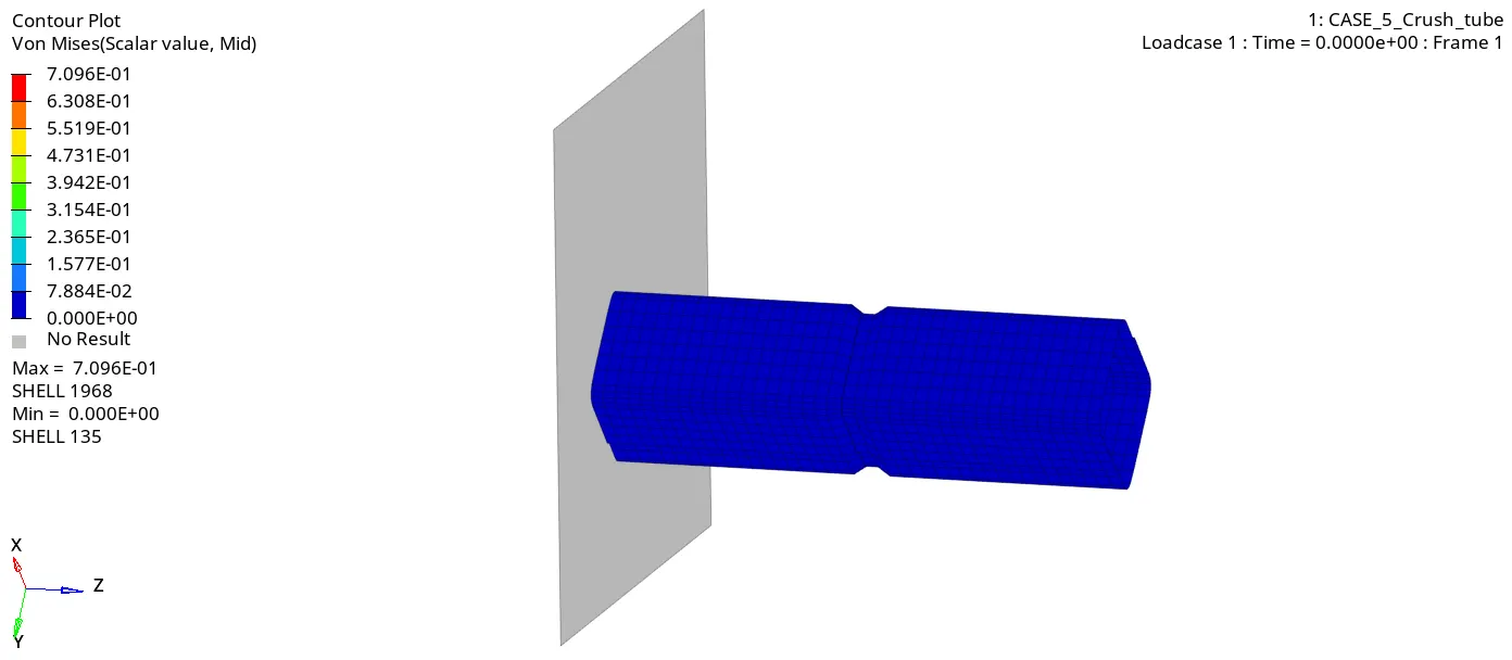
Contour plot for Von mises stress:

Stress generated up to 7.096E-01 GPa only from zero at the beginning. Stress is a little higher in this case because we kept the notch in the middle of the model.

A component starts deformation at the middle where the notch is located because there's less resistance strength on that area and also some stress flow interruption has happened.

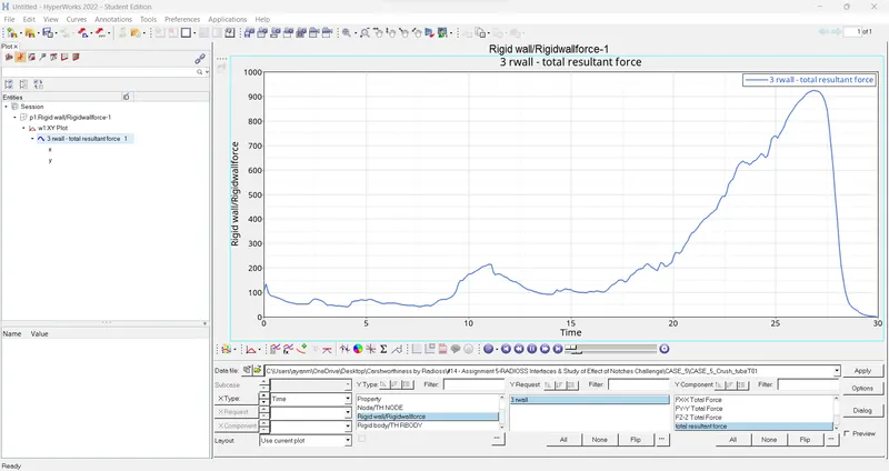
Rigid wall total resultant forces:

There's no change in the total resultant force plot if run the model is with or without the notch.

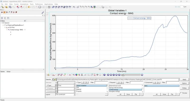
Contact energy:

There's no change in the contact energy plot if run the model with or without the notch.

Internal energy:

There's no change in the Internal energy plot if run the model with or without the notch.

CASE 6:

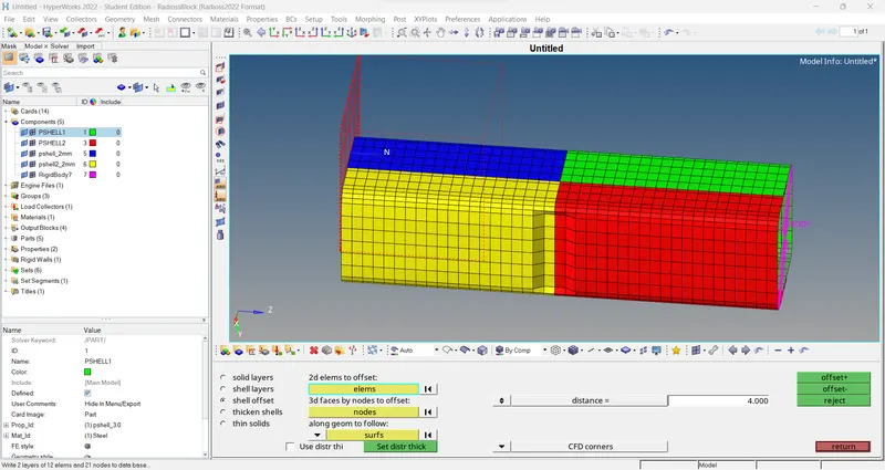
In this case, we have to create a new notch with nodes only from opposing 2 faces and run.

To create the notch in the middle, Element offset option under 2D is used.

Go to 2D > elem offset > shell offset > 2D elems to offset > select 1 layer of elements > put distance > offset+

In this case, errors are very close to 0 which means it's acceptable. It didn't take more cycles as compared to previous cases.

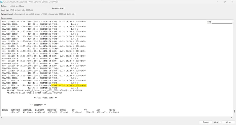
From the OUT file,

• energy error = 0% to -1.3%
• mass error = 0.00

Since the energy and mass error are within the acceptable range, the model is stable.

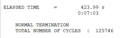
Now the time for simulation and number of cycles taken to complete the simulation is also noted from the OUT file.

After completion of solving, switch to "Hyperview" from the "HyperMesh" section.

Select the appropriate file in an "h3d" format and open the same file in the Hyperview interface.

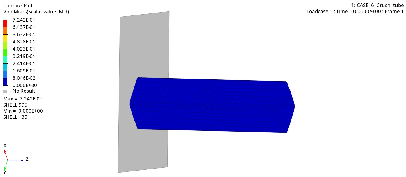
Contour plot for Von mises stress:

Stress generated around 7.242E-01 GPa only from zero.

A component has been starting the bending deformation at the middle on the flat side. At the end of the simulation, a model has ended up inclined in shape.

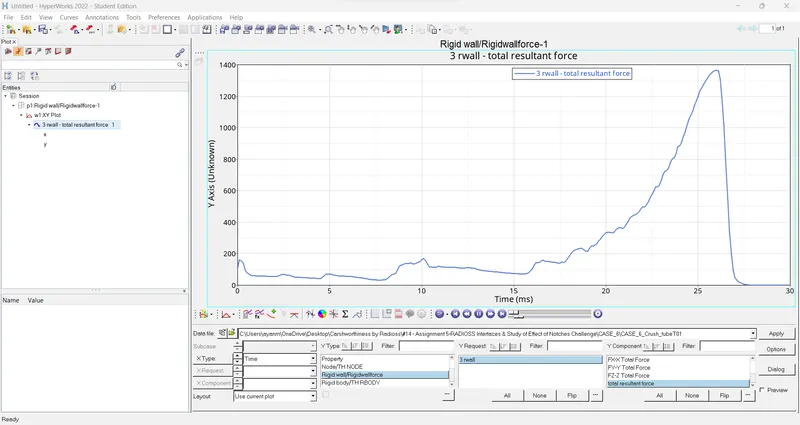
Rigid wall resultant forces:

In this case, a maximum resultant force is lesser than in previous cases. Up to 15 ms, forces are varying gradually with a lesser rate. After 15 ms, forces are varying linearly up to 27 ms with a maximum value of around 1400. Then, it suddenly falls down to 0 at the termination time.

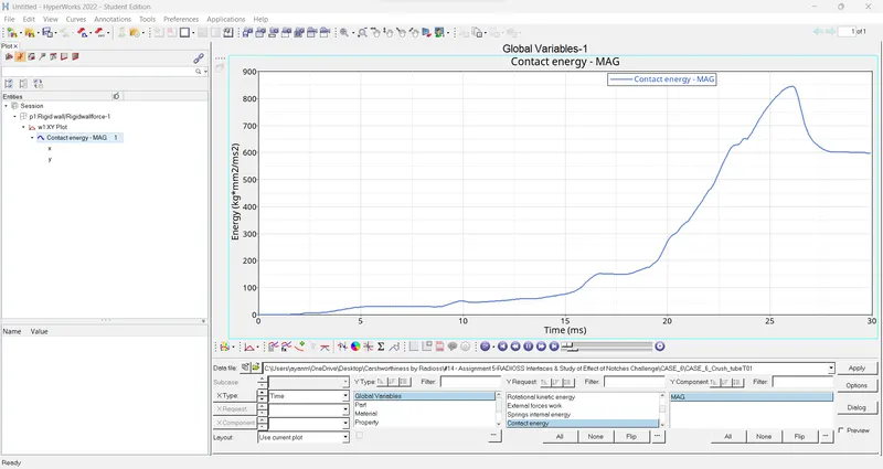
Contact energy:

Contact energy also is varied as compared to previous cases. A maximum value reaches around 850 in this case.

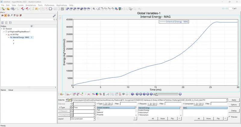
Internal energy:

There's no change in the Internal energy plot in this case.

> Comparison for all CASEs plots....

> plot Rigidwall force for all Cases..

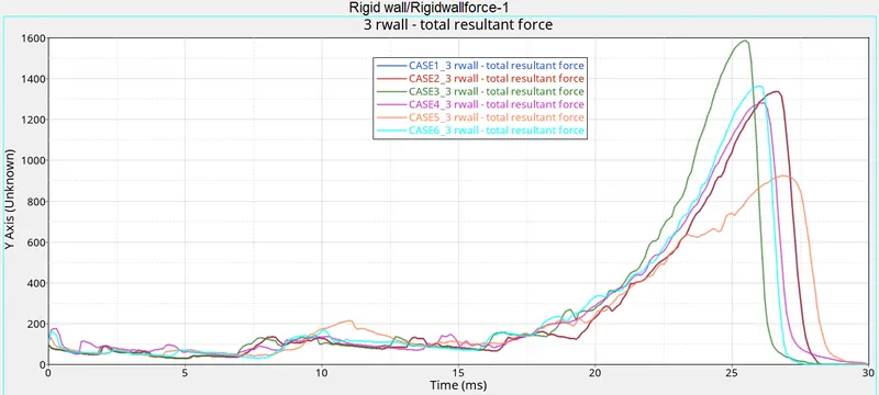
> plot Contact Energy for all Cases..

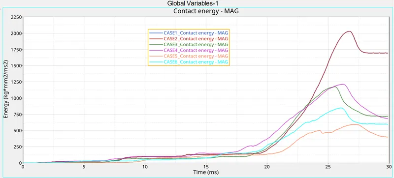
> plot Internal Energy for all Cases..

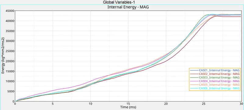
CONCLUSIONs:

Cases\Parameters	Case 1	Case 2	Case 3	Case 4	Case 5	Case 6
Contact Interface Type	TYPE 7	TYPE 7	TYPE 11 (added)	TYPE 11 (added)	TYPE 11 (added)	TYPE 11 (added)
Changes on the model	No changes	Change into "Incti = 6"	Change into recommended parameters	Removed notches and boundary condition	Created a new notch in the middle.	Create a notch on opposing faces only.
Energy Errors in %	-3.8	-3.8	-1.6	-1.5	-0.9	-1.3
Maximum Stress in Mpa (Von Mises)	0.7352	0.7352	0.7783	0.7266	0.7096	0.7242
Number of cycles	83469	83469	128088	146924	140877	125746
Internal Energy (kg*mm2/ms2)	42273	42265	43021	42998	43268	43262
Rigid wall forces (kN)	1338	1338	1588	1281	925	1364
Contact energy (kg*mm2/ms2)	2029	2029	1172	1212	593	845

TYPE 7 is a variable stiffness and its contact work node to surface. When we use this, it might be slave edge will penetrate across the master surface.

TYPE 11 is also being a variable stiffness, but its contact works edge to edge. When we use this type, it will not allow penetrating across the element.

Why there is a change in internal energy?

In case 1, we have used default parameters which are available in the Type 7 contact card. but when we added Type 11 that will lead to an increase in the internal energy from the beginning time itself. Because it has a more inertial force on it. Rest of the cases, the internal energy is close to similar than the previous one because we kept the parameter as recommended one.

How does notch affect the results?

A notch means is basically a change in the cross-section of the component. When we keep the notch in the components, by results in uneven stress distribution. When we use the notch in the component, that will lead to an increase the internal stress generation.

In case 4, we didn't keep the notch in the component. As a result, a component experienced less stress generation as compared to all other remaining cases that have notches on it.

Notches are the regions where deformations happen first, due to them being regions of stress concentration. But it does help to control and predict the location of deformations. This in turn plays a role in how the absorbed energy spreads throughout the tube. A notched tube results in higher contact forces but a smoother transmission of load.

In this assignment, different types of contacts were used to analyse the simulations of the crash tube. Under a constant load, the behaviour was observed by varying the geometry through the removal and creation of notches.