Week 3 - Solving second order ODEs

SECOND ORDER ODEs:

AIM: To solve second order ordinary differential equation using MATLAB.

OBJECTIVE:

1. To create a plot between angular velocity and displacement of simple pendulum by using ode45 in MATLAB.
2. To create an animation of simple pendulum by using second order differential equation by using ode solver function.

THEORY:

Ordinary Differential Equation (ODEs) – An ordinary differential equation (ODE) is a differential equation containing one or more functions of one independent variable and the derivatives of those functions. The term ordinary is used in contrast with the term partial differential equation which may be with respect to more than one independent variable.

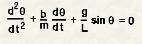
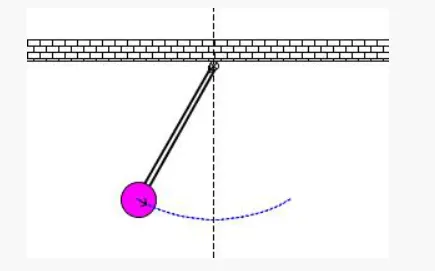
Simple Pendulum – The simple pendulum is an idealized mathematical model of a pendulum. This is a weight (or bob) on the end of a massless cord suspended from a pivot, without friction. When given an initial push, it will swing back and forth at a constant amplitude. Real pendulums are subject to friction and air drag, so the amplitude of their swings declines.

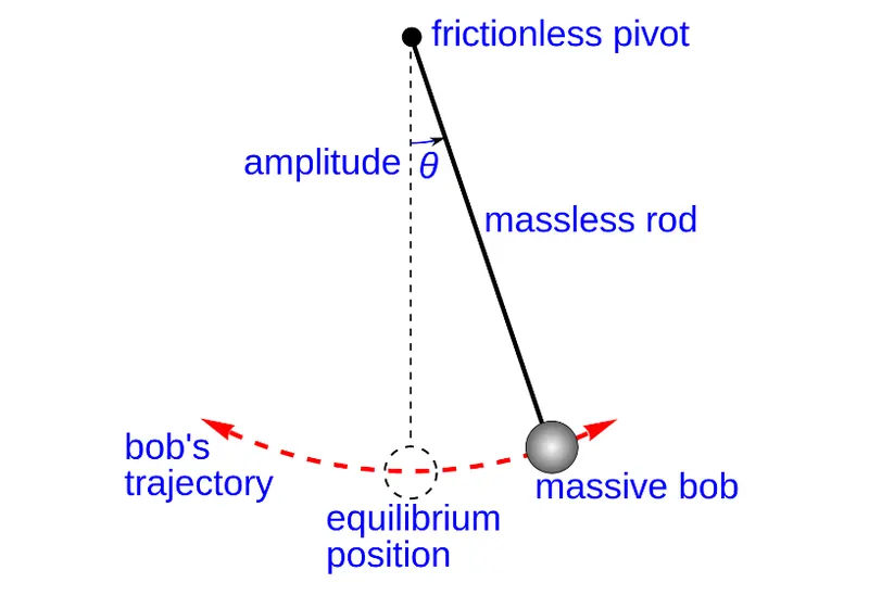
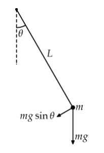
The point from which the bob is suspended is known as point of suspension. Weight of the bob acts vertically downwards and the tension acts vertically upwards, so, the bob comes under equilibrium position and the bob starts oscillating if even smaller external force is applied.

MATHEMATICAL EQUATIONs:

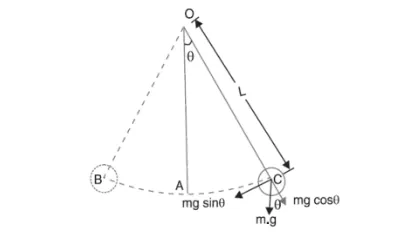
`θ`is the angle made by the movable link with vertical axis.

'L' is the length of the movable rod

'm' is the mass of bob, b is damping coefficient of the system.

1. `(d^2 θ)/(dt^2 )+b/m×d(θ)/dt+g/L sin⁡θ=0`second order ODE………(1)

To solve this ODE we need to reduce the order of equation into lower order,

Let , `θ=θ1`

So this implies`d(θ)/dt=d(θ_1 )/dt=θ_2` ……….(2)

Therefore,`(d^2 θ)/(dt^2 )=(d^2 θ_1)/(dt^2)=d(θ_2 )/dt` ……………(3)

Putting the value of (2) and (3) in (1), we get-

`(d^2 θ_1)/dt+b/m×d(θ_1)/dt+g/L sin⁡[θ_1 ]=0`

Therefore,`d(θ_2 )/dt+b/m (θ_2 )+g/L sin⁡[θ_1 ]=0`

We got, `d(θ_2 )/dt=-b/m (θ_2 )-g/L sin⁡[θ_1 ]`

The simple differential equations are written in the form of a matrix,

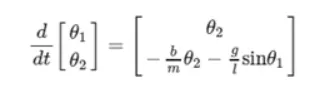
By using the above equation and the ode45 solver we can animate the simple pendulum in MATLAB by writing a code.

PROCEDURE:

Given details are simulate the motion between 0-20 sec, for angular displacement =0, angular velocity= 3rad/sec at time t=0;

L= 1 meter

M= 1 kg

b= 0.05 N-m/s

g= 9.81 m/s²

CODE EXPLANATIONs:

1. Start programming in MATLAB with these three commands, as all the previous calculations are erased.

Clear all: for clears all the data stored in the workspace previously.

Close all: for closes all the previous figures and plots.

clc: for clears the command window.

2. Now give inputs for the simple pendulum are specified and the b (damping coefficient) = 0.05 (N-m/s), g (acceleration due to gravity) = 9.81 (m/s), l (length of the string) = 1 (meter), m (mass of the bob) = 1 (kg). and

Simulate Angular velocity = 3rad/sec at time t = 0, the motion between 0-20 sec for angular displacement= 0.

3. ’t_span’ is a command used in the ode45 solver which specifies the time span of the iterations that are going to solve the ordinary differential equation.
4. ‘ode45’ is a function in Matlab that solves ordinary or partial differential equations using a numerical method. In this problem the highest order is 2 . So, we have to take two constant values so that the equation is changed to simple differential equation.

The function should take at least 2 inputs to solve the equation to the approximate result.

5. The ode45 function has a syntax in which we need to specify which should be ‘t’ and ‘y’ & the output may be of (t,y,args) and a timespan for the function to work and the initial value of the equation.
6. Syntax of a ode45 solver [t,results]= ode45(@(t,y) ode(t,y,args), t_span,y0).

I use [t,results]=ode45(@(t,theta)ode_func(t,theta,b,l,m,g),t_span,theta_0);

After this ‘ode45’ and corresponding ‘ode_func’ functions call in main program...

7. Figure1 is going to tell how the damping is done for the pendulum, the angular velocity and displacement will come to rest at end of the function.
8. Plotting the values for the angular velocity and the displacement by using plot command, the label command is used to label the X & Y axis.
9. Legend command is used to label the angular velocity and the displacement.

10. For getting the accurate simulation of the simple pendulum corresponding to the second order ODE with damping we need to use the loop statements to creates the specified set of points to keep the bob at different locations.
11. x0 and y0 be the fixed point at one end of the string and x1 and y1 be different position of the bob.
12. At each and every point of the bob, the ‘ct’ command which is used to count each and every position and stores the data.
13. For figure2 plot coordinates for the motion path of pendulum.
14. Marker command is used for making bob of the pendulum, the axis is fixed using axis command. The counter command is used to make the value changes in each for loop.
15. Then videoWriter command is used to create the video file.

Movie(M): to create a flim of the stored data of the motion of the pendulum.

videoWriter: this command specifies the name of the file and type of data is stored in it.

‘open’: this command is used to open the file where the video is going to store.

writeVideo: is used to create the video animation by using ‘M’ file.

close: this command is used to close the video file.

1. CODE FUNCTION (ode_func) OF ODE45 FOR MAIN PROGRAM:

function [dtheta_dt] = ode_func(t,theta,b,l,m,g)
theta1 = theta(1);
theta2 = theta(2);

dtheta1_dt = theta2
dtheta2_dt = (-(b/m)*theta2 - (g/l)*sin(theta1));
dtheta_dt = [dtheta1_dt; dtheta2_dt];

end

1. MAIN PROGRAM:

%Solving the Second order ODE and show the animation
clear all
close all
clc

b=0.05;  %damping coefficient
l=1;     %length of pendulum in meter
m=1;     %mass of bob in kg
g=9.81;  %gravity in m/s^2

%Initial condition
theta_0=[0;3];

% Time span
t_span=linspace(0,20,500);

%ode45 function to Solve second order ODE.
[t,results]=ode45(@(t,theta)ode_func(t,theta,b,l,m,g),t_span,theta_0);

figure(1)
plot(t,results(:,1))
hold on
plot(t,results(:,2))
xlabel('Time')
ylabel('Velocity')
title('Fig1: Time vs Veolocity graph represent Displacement & Velocity')
legend('Displacement','Angular Velocity')
grid on
hold off

displacement=results(:,1);
velocity=results(:,2);

%fixed coordinates
x0=1;
y0=1;
ct=1;

for i=1:length(displacement)

    %coordinates
    x1=1-l*sin(displacement(i));
    y1=1-l*cos(displacement(i));

    figure(2)

    %plot fixed link
    plot([0 2],[1 1],'linewidth',10,'Color','r')
    hold on
    plot([1 x1],[1 y1],[x1 x1],[y1 y1],'-o','markersize',20,'markerfacecolor','g','LineWidth',4)
    plot(x0,y0,'-o','markersize',5,'markerfacecolor','b')
    title ('fig2:animation of a simple pendulum')
    %axis setting
    axis([0 2 -0.5 2])

    M(ct)=getframe(gcf);    %to change the frame of the movie.
    ct=ct+1;
    hold off
end
movie(M)                    %for creating animation video.
videofile=VideoWriter('simple pendulum.avi','Uncompressed AVI');
open(videofile)             %open the videofile while running the code.
writeVideo(videofile,M)     %for writing the video file.
close(videofile)            %for closing the video file after code run.

OUTPUT:

The plot is representing the angular acceleration and displacement of the motion of simple pendulum. (fig: time vs. velocity)

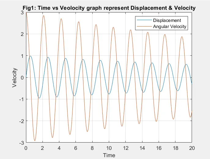
The blue curve is the displacement where it starts from zero, and red one is the angular velocity which starting at 3(rad/sec).

At the end of the t_span both the displacement and angular velocity becomes zero and motion of simple pendulum becomes zero which becomes rest.

ERRORs:

In line 51 plot typing error '-0' instead of '-o' .

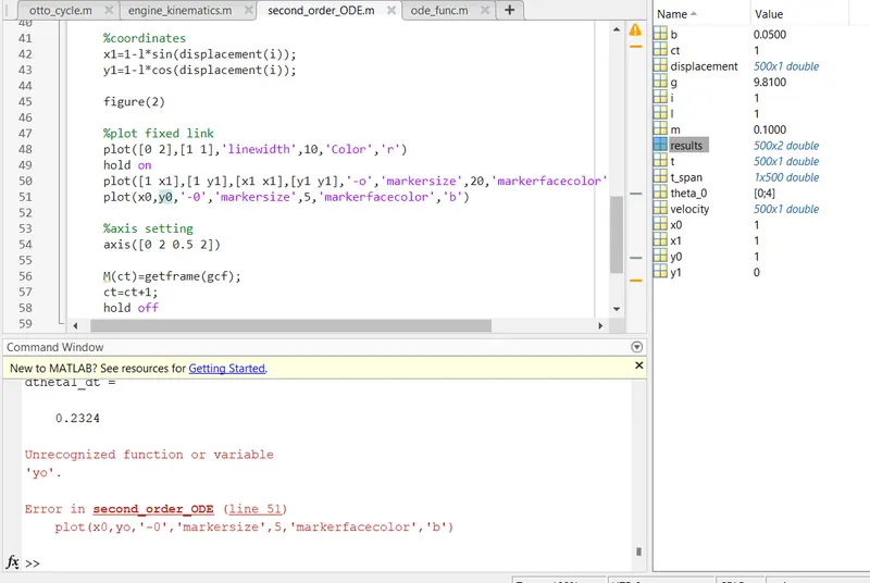
Solution: Analysis it from command window and replace '-0' to '-o' and run it again.

CONCLUSIONs:

1. We can analysis the Displacement and Angular Velocity from Velocity vs Time diagram.
2. We have animated the simple pendulum using the ode45 solver where the second order is reduced to a simple differential equation where it is easy to solve the given equation.
3. The animation is made using the different points of the bob and the motion of the simple pendulum is created.

Position of the simple pendulum setup:

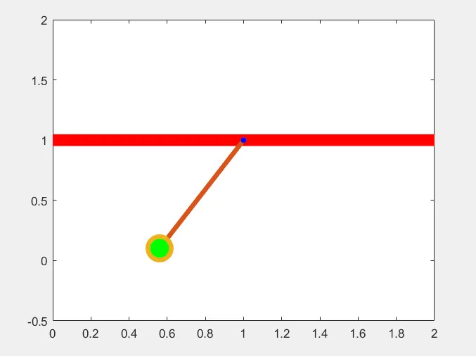
Animation of simple pendulum:

https://drive.google.com/file/d/1e3LQvnc7fE9Z2G8u-AXLxlHnCcXvbi2e/view?usp=sharing

https://drive.google.com/file/d/1e3LQvnc7fE9Z2G8u-AXLxlHnCcXvbi2e/view?usp=sharing