week-11 Joint creation and Demonstration

#12 // week- 11 Joint creation and Demonstration.

Aim: To demonstrate revolute, cylindrical, spherical, and translational joints between two rigid bodies also with two deformable bodies using the *CONSTRAINED_JOINT keyword.

Objective:

To create four types of joints using constrained extra nodes and constrained nodal rigid keywords with the help of Ls-Dyna.

Theory:

The revolute joint –>

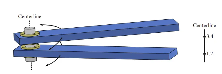
• The revolute joint in ls-Dyna is also called a hinge joint and has only one degree of freedom (Pure rotational motion along a common axis).
• The above figure shows a revolute joint with two nodal pairs formed by nodes 1, 2, and 3, 4. The nodal points 1 and 2 should coincide in the initial configuration. similarly, nodes 3 and 4 should satisfy this condition. Nodes 1 and 3 should belong to one body(A) and nodes 2 and 4 should belong to another body(B).
• For rigid bodies use *CONSTRAINED_EXTRA_NODES to include the joint nodes (nodes1,2,3,4 shown above) to the respective rigid bodies. For deformable bodies, the joint nodes should be a part of *CONSTRAINED_NODAL _RIGID_BODY which has some shared nodes with the deformable body.

The cylindrical joint –>

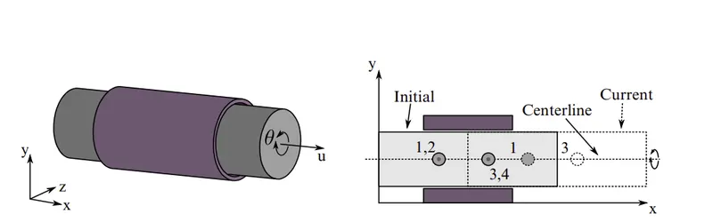
• This joint is derived from the rotational joint by relaxing the constraints along the centreline. This joint admits relative rotation and translation along the centreline.
• The above figure shows a cylindrical joint with two nodal pairs. Here nodes 1 and 2 should coincide with each other and node 3 and 4 should coincide with each other. It should be assigned in such a way that nodes 1 and 3 belong to the inner cylinder and nodes 2 and 4 belong to the outer cylinder.

The spherical joint –>

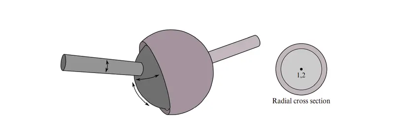
• The relative motion of the rigid bodies is constrained so that nodes that are initially coincident remain coincident. In the above figure, the socket’s node is not interior to the socket—LS-DYNA does not require that a rigid body’s nodes be interior to the body.
• This joint admits rotational motion only.
• Here node 1 belongs to part A (outer) and node 3 belongs to part B (Inner).

The translational joint –>

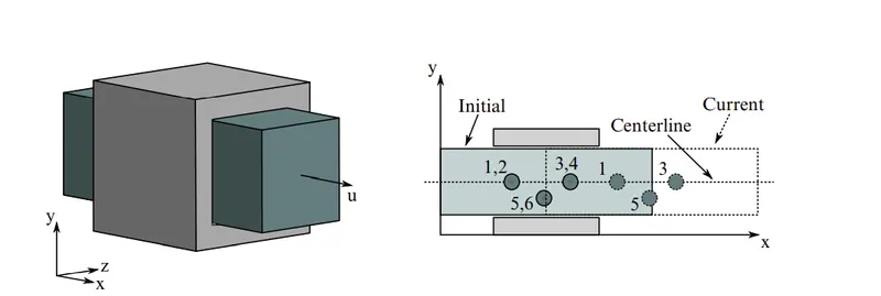
• The translational joint has only one translational degree of freedom and zero rotational degrees of freedom.
• This is a cylindrical joint with a third pair of off-centreline nodes which restrict rotation. Aside from translation along the centreline, the two rigid bodies are stuck together.
• Here the nodes (1,2) have coincided with each other. Similarly, the nodes (3,4) also (5,6) are coincided with each other as shown in the figure.

Procedure:

Revolute Joint:

/ Creating geometry for revolute joint -

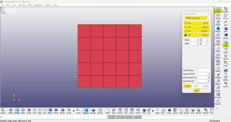
• Two separate shell elements are created using the Element and mesh > Shape Mesher option available in LS-PrePost. Select the entity as 4N and assign the node coordinates for the shell element with the required mesh density.
• Some free spaces (here 30mm) are kept in between the two pairs for a better presentation of a revolute joint.

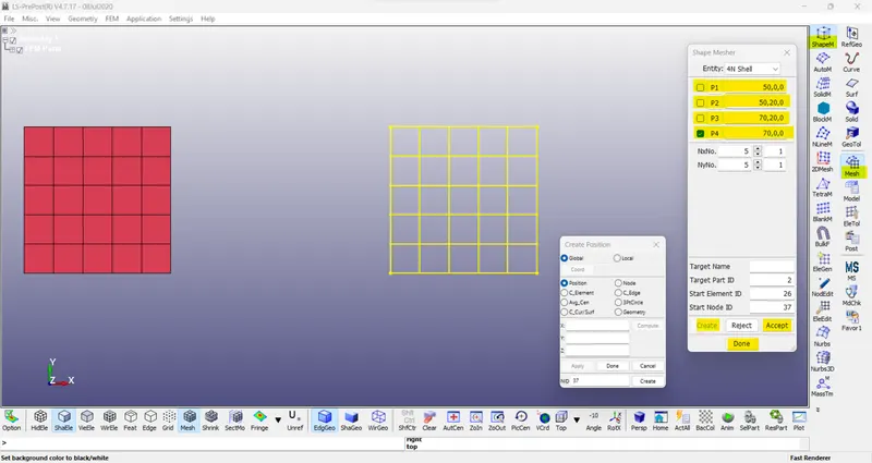
1. Revolute joint between two rigid bodies using *CONSTRAINED_EXTRA_NODES.

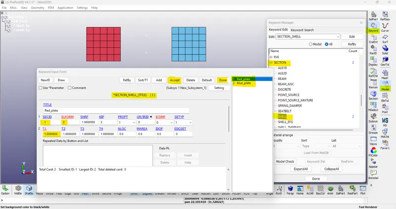
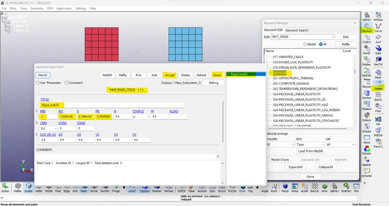
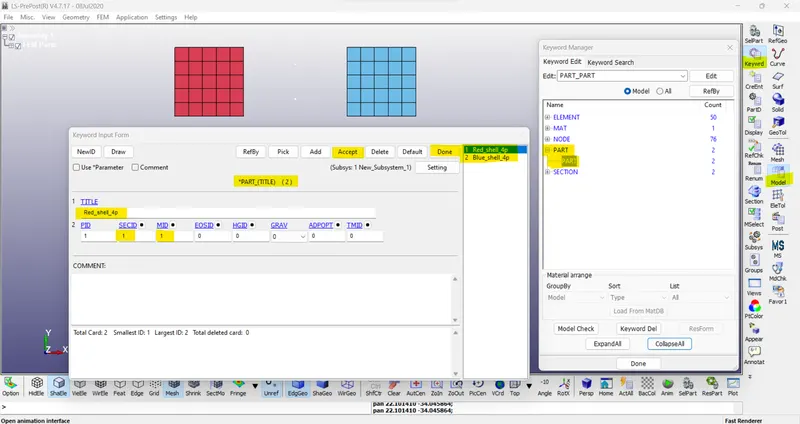
• Define a section property as a shell for created elements by using the *SECTION_SHELL keyword. Also, define a rigid material using the *MAT_RIGID keyboard. Use a reasonable value while defining the material properties. Define the respective MATID and SECID for the two PARTs.

Section-

Material-

PART-

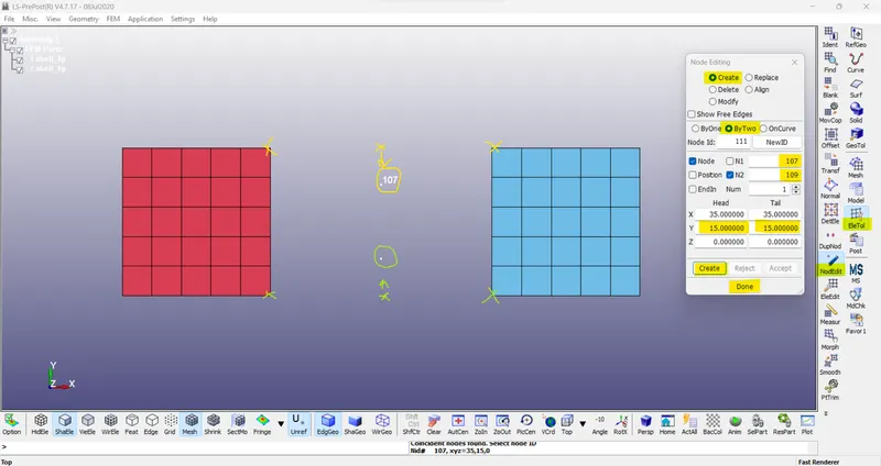
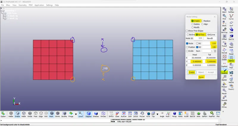
• Create four extra nodes manually which are further needed to be associated with two parts for making a revolute joint. Create nodes by Element Tool > Node Editing option to give distinct node ids for all four nodes. Here four nodes are numbered 107,108,109,110.
• The nodes 107 and 109 are coincident and nodes 108 and 110 are also coincident.

• Now create a new node-set, where nodes 107 and 108 belong to one node-set, and nodes 109 and 110 belong to another node-set. This can be done using Create entity > Set Data > *SET_NODE > Create option.

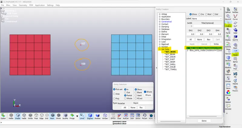
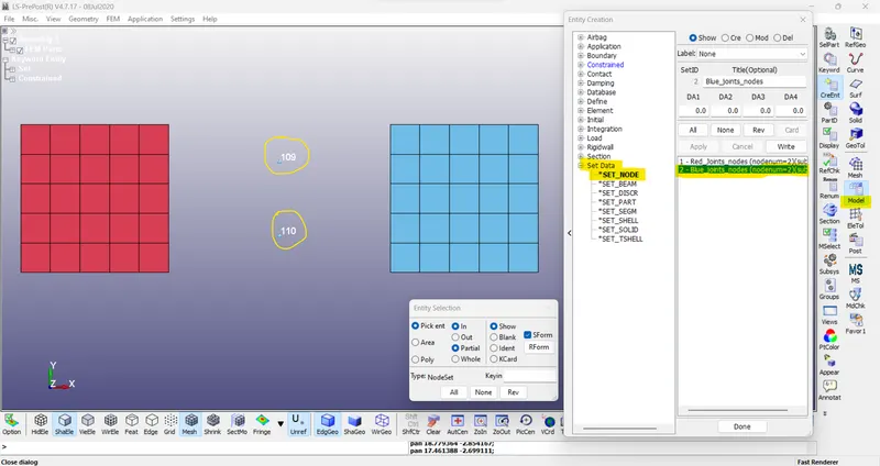
• These newly created nodes are in the space and do not belong to any of the parts now. So, for associating these nodes with part 1 and part 2, *CONSTRAINED_EXTRA_NODES_SET is used.
• Here nodes 107 & 108 belong to part 1 and 109 & 110 belong to another part 2.

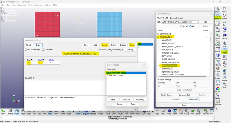
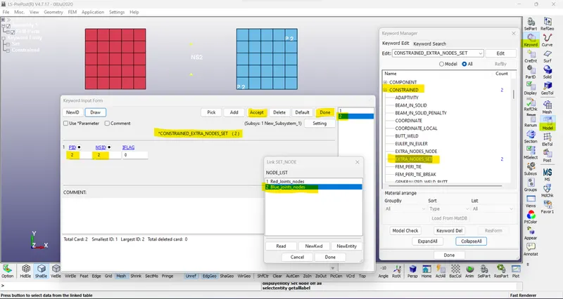
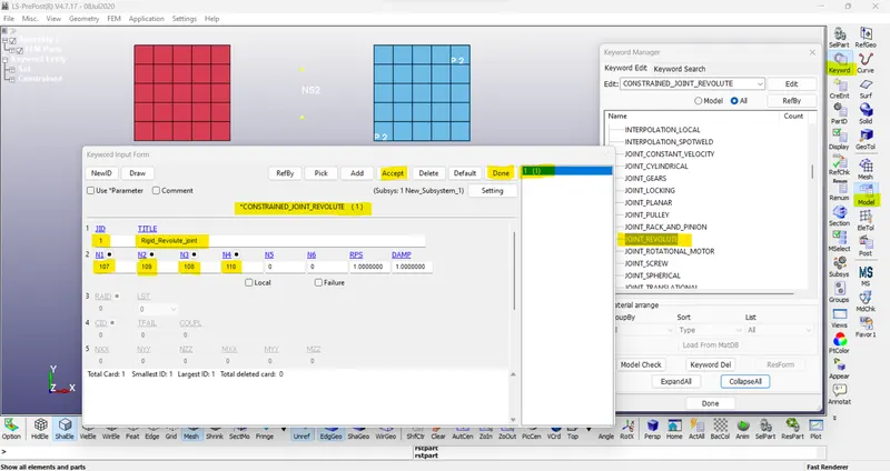
• Now, the revolute joint is defined by using the *CONSTRAINED_JOINT keyword. Four nodes should be defined to create a revolute joint. N1 and N3 belong to body 1 and N2 and N4 belong to body 2.

• Now, to make this revolute joint work, a few boundary conditions are essential. So, a displacement along the Z direction is applied to one of the nodes in part 2. This is defined by the *BOUNDARY_PRISCRIBED_MOTION keyword. The z-translational DOF is kept free by assigning DOF= 3 in the keyword.

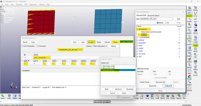
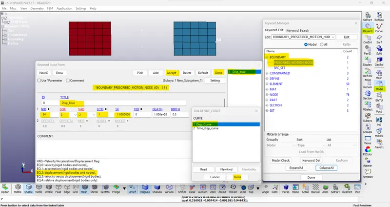
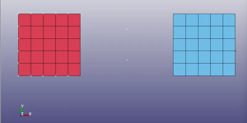
• Single point constraint (SPC) is also used to fix part 1 at its position. Several nodes on the edges of part 1 are selected and assigned *BOUNDARY_SPC. The figure below shows (left part) fixed nodes in part 1 which is marked in green color and a node is selected to give displacement in part 2 which is denoted in red color.

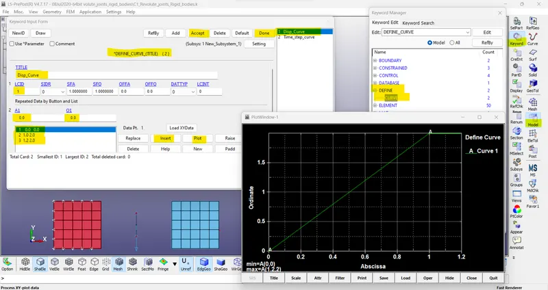
• A displacement curve was also defined for the prescribed motion keyboard which is defined by LCID.

Control-cards:

1. Control cards Such as Control Termination, Control Implicit Auto, Control Implicit General, And Control Time step Is Defined.
2. As Displacement is given Implicit Solver Is chosen for better results.

• Control Termination Card Is defined With the Termination Time 1ms.
• Database Binary D3Plot is defined to print the Results at 0.1ms in each interval.
• Control Timestep Card is defined For Stable Time Step.

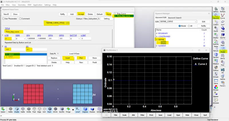
• *CONTROL_TIMESTEP card is used and a load curve which is shown below is assigned through the LCTM option. The timestep calculated by the solver for these rigid bodies and this mesh size is large enough hence for more stability.

Post-processing:

Results:

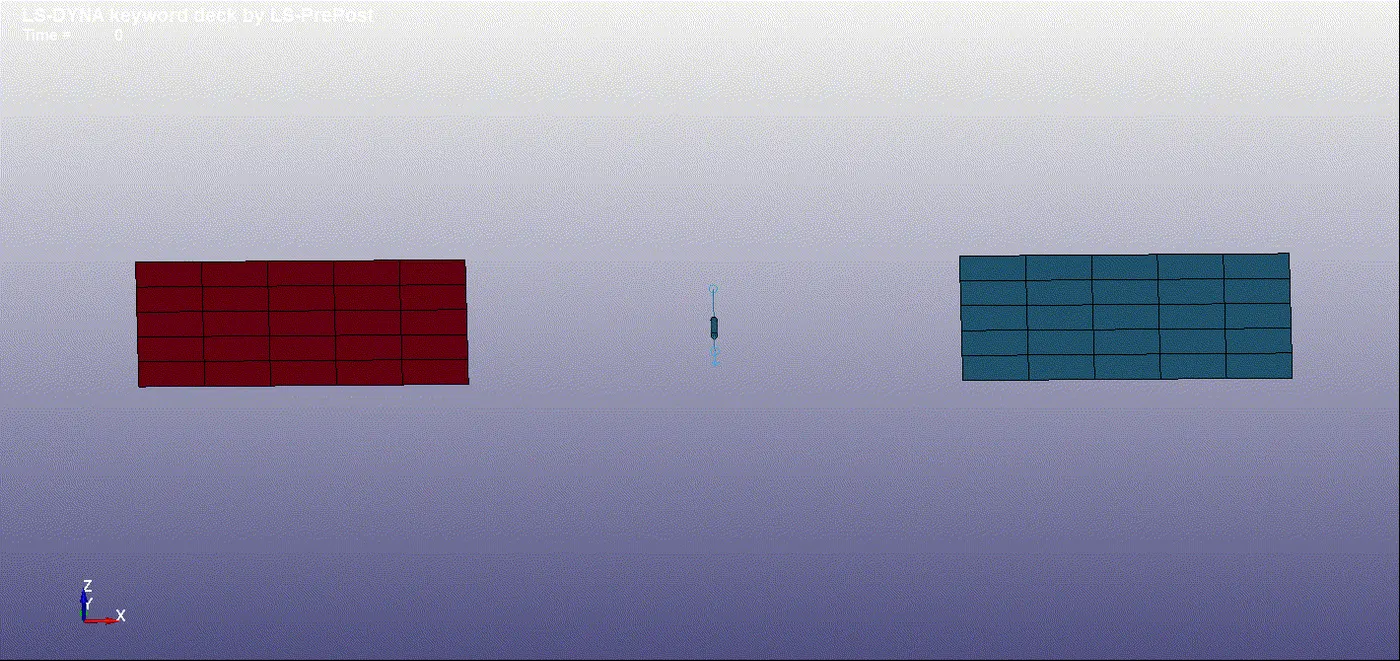
• The revolute joint between two Rigid bodies using *CONSTRAINED_EXTRA_NODES is shown below.

2. The revolute joint between two deformable bodies using CNRBs.

• Here also two separate shell elements are created as that of the above model.
• Four noded revolute should be created with the help of *CONSTRAINED_NODAL_RIGID_BODY(CNRB) when needed to model a revolute joint between two deformable bodies.
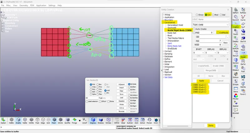
• At first, four nodes are created which would be further used to create CNRBs. Create nodes by Element > Tools > Node Editing and give distinct node IDs for all four nodes.
• To create a CNRB, go to Create Entity > Constrained > Nodal Rigid Body (CNRB) > Create. uncheck the CrePNode option which will disable the creation of PNODE at the mass center of the selected nodes.

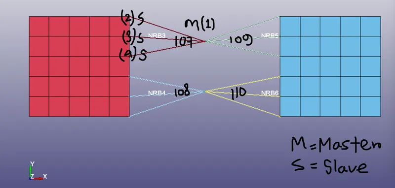
• For deformable bodies, the material is assigned using the *MAT_ELASTIC keyword. Here also the material card and section card are finally assigned to the part id.

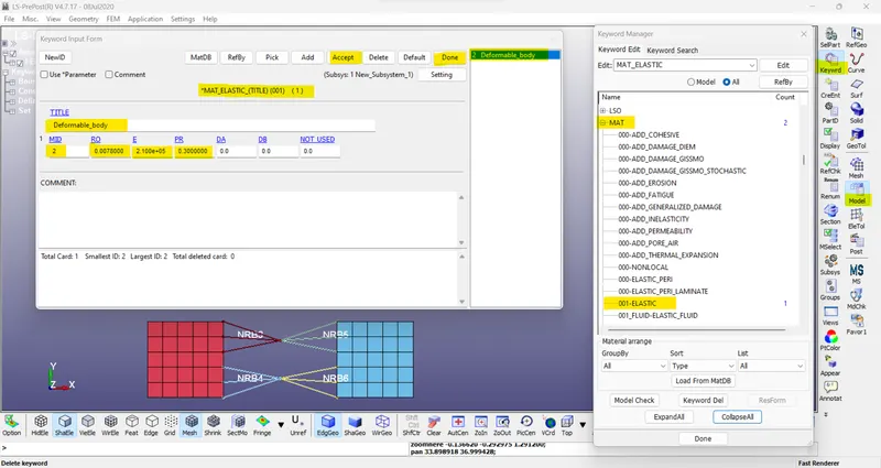
• Revolt joint is defined by using the *CONSTRAINED_JOINT keyword. Four nodes should be defined to create a revolute joint. Here N1 and N3 belong to part A and N2 and N4 belong to part B.

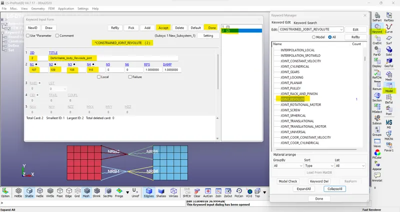
• Here *CONSTRAINED_EXTRA_NODES should not be used.
• The same boundary conditions, displacement, and time step curve are used in this analysis which is similar to the previous section.

Post-processing:

Results:

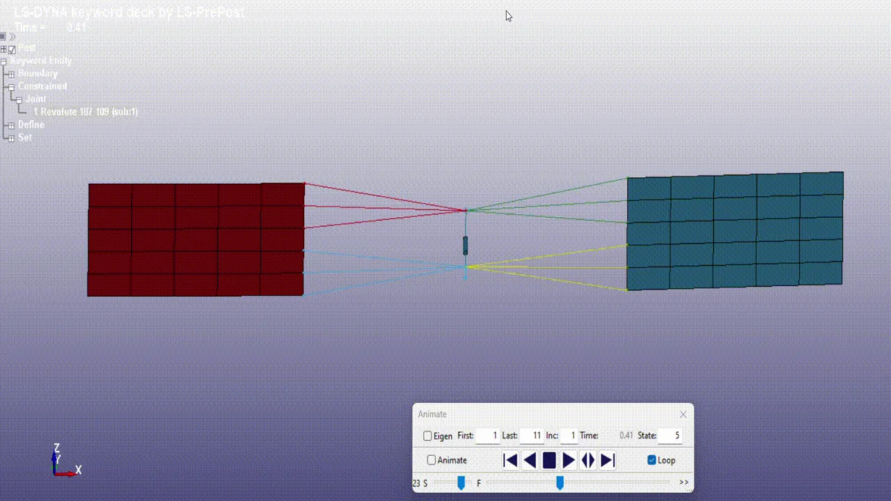
• The revolute joint between two deformable bodies using *CONSTRAINED_NODAL_RIGID_BODY (CNRB) is shown below.

The cylindrical joint:

/ Creating geometry for cylindrical joint -

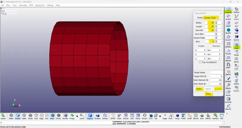
• Two cylindrical shell elements (inner and outer) are created using the Mesh > Shape Mesher > Entity > Cylindrical shell option available in LS-PrePost.

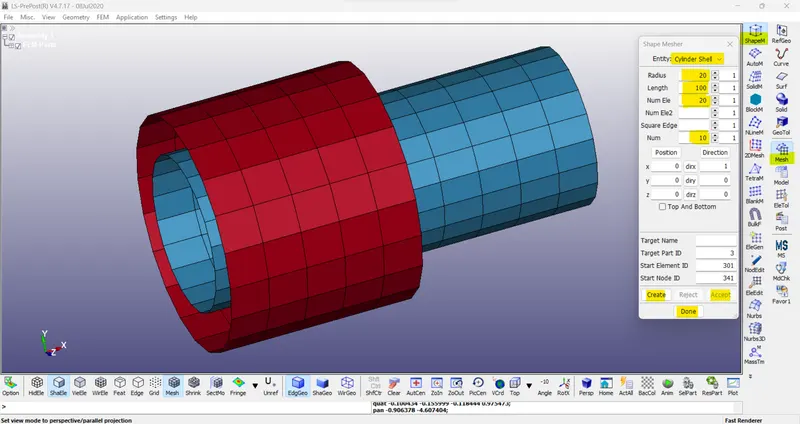
1. Cylindrical joint between two rigid bodies using *CONSTRAINED_EXTRA_NODES.

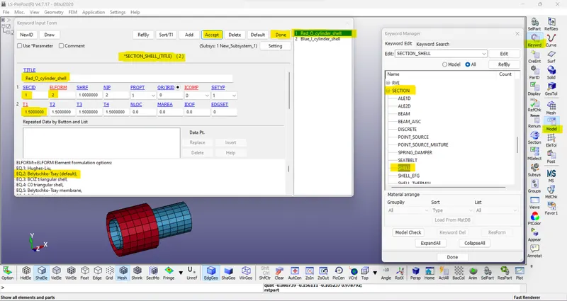
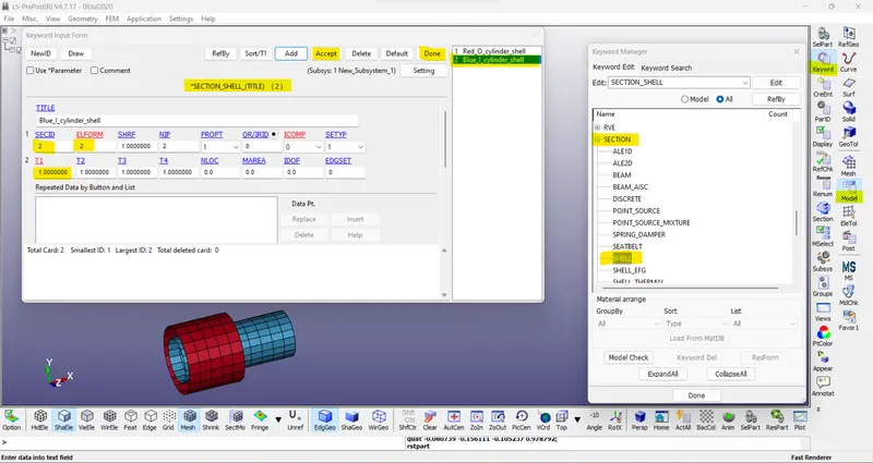
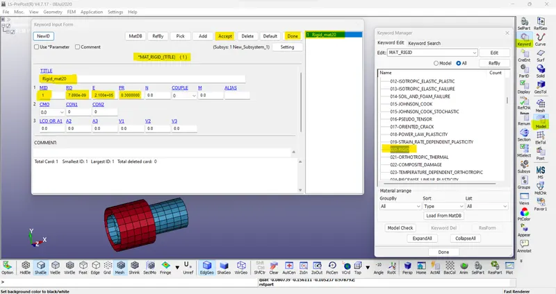
• Define a section property as a shell for created elements by using the *SECTION_SHELL keyword. Also, define a rigid material using the *MAT_RIGID keyboard. Use a reasonable value while defining the material properties. Define the respective MATID and SECID for the two parts.

Section-

Material-

PART-

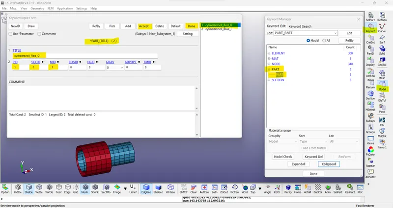
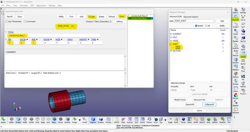
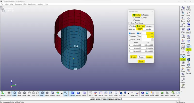
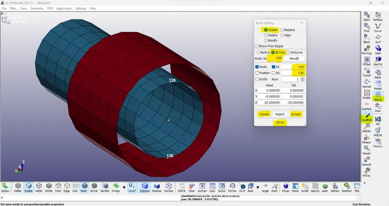
• Create four extra nodes manually which are further needed to be associated with two parts for making a cylindrical joint. Create nodes by Element Tool > Node Editing option to give distinct node ids for all four nodes. From there use the 'by two' option to create the node in the center of the cylinder.
• (Note- 1007,1008 front side with same nodes & 1009, 1010 back side same nodes.)

• Now create a new node-set in which nodes 1007 and 1009 belong to the inner cylinder (Blue) and nodes 1008 and 1010 belong to the outer cylinder (Red) as discussed above. This can be done using Create entity > Set Data > *SET_NODE > Create option.

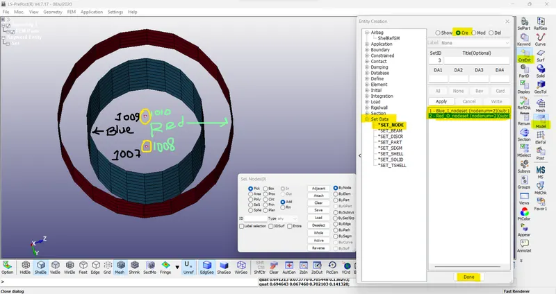
• These newly created nodes are in the space and do not belong to any of the parts now. So, for associating these nodes with part 1 and part 2, *CONSTRAINED_EXTRA_NODES_SET is used.

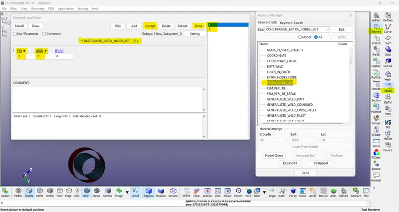
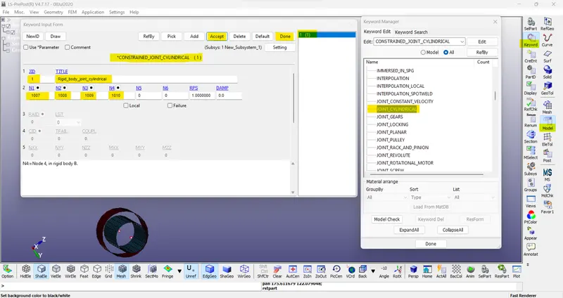
• Now, the cylindrical joint is defined by using the *CONSTRAINED_JOINT_CYLINDRICAL keyword. Four nodes should be defined to create a cylindrical joint. N1 and N3 belong to body 1 and N2 and N4 belong to body 2.

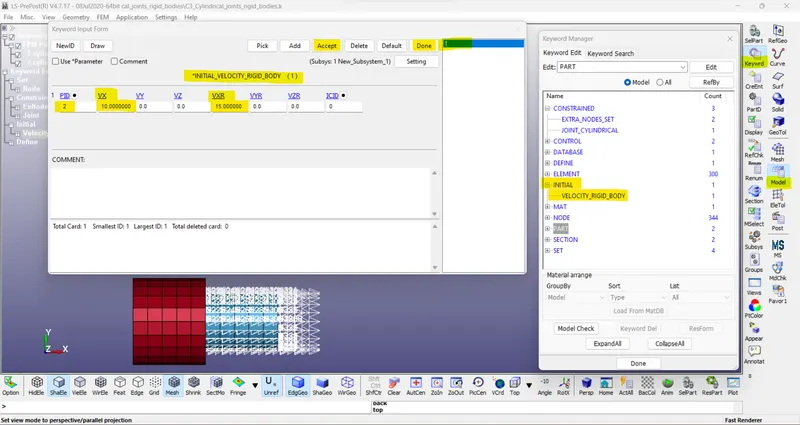
• Now an *INITIAL_VELOCITY_RIGID_BODY card is created to assign the velocity by selecting the required PID. Since the cylindrical joint possesses both translational and rotational motion about a particular axis, we may assign it accordingly.

Control-cards:

1. Control cards Such as Control Termination, And Control Time step Is Defined.
2. As INITIAL_VELOCITY_RIGID_BODY with a small run time is given Explicit Solver Is chosen for better results.

• Control Termination Card Is defined With the Termination Time 1ms.
• Database Binary D3Plot is defined to print the Results at 0.1ms in each interval.
• Control Timestep Card is defined For Stable Time Step.

• *CONTROL_TIMESTEP card is used and a load curve which is shown below is assigned through the LCTM option. The timestep calculated by the solver for these rigid bodies and this mesh size is large enough hence for more stability, we use smaller time steps for explicit analysis.

Post-processing:

Results:

• The cylindrical joint between two rigid bodies using *CONSTRAINED_EXTRA_NODES is shown below.

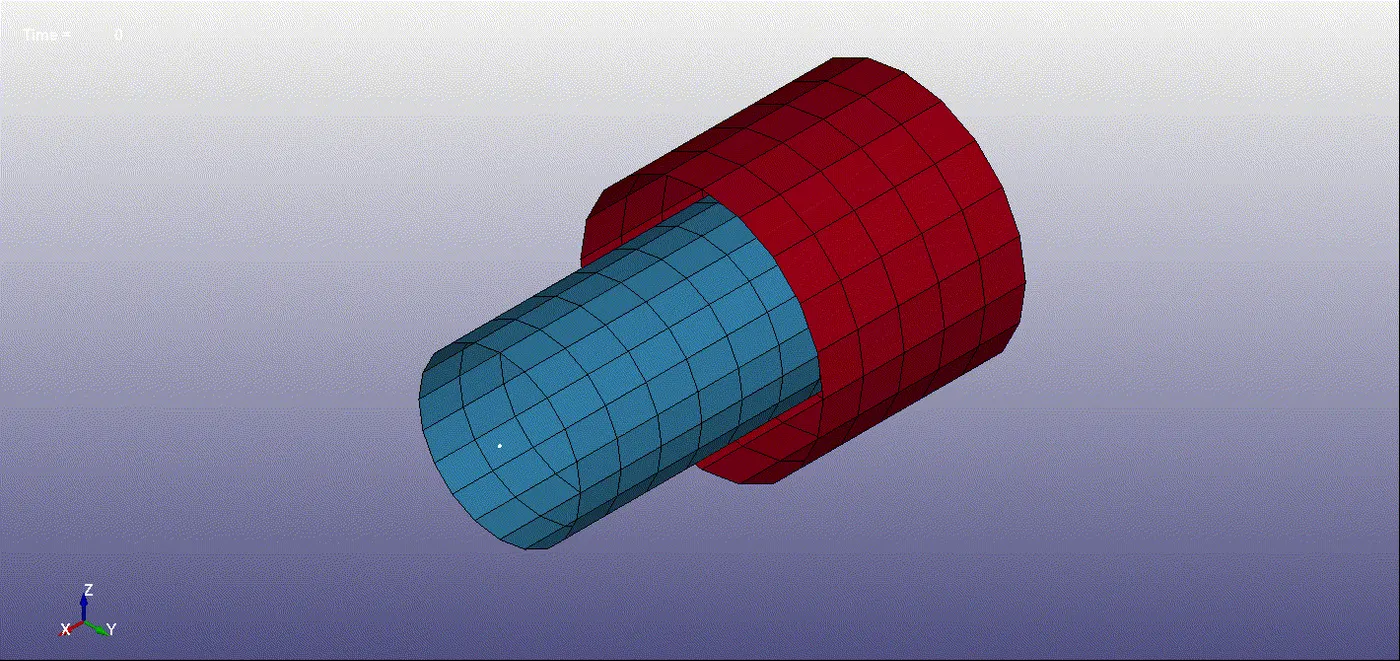
2. The cylindrical joint between two deformable bodies using CNRB

• The cylindrical joint between two deformable joints is created with the help of *CONSTRAINED_NODAL_RIGID_BODY(CNRB).
• At first, four nodes are created which would be further used to create CNRBs. Create nodes by Element > Tools > Node Editing and give distinct node IDs for all four nodes.
• To create a CNRB, go to Create Entity > Constrained > Nodal Rigid Body (CNRB) > Create. Toggle off the CrePNode option which will disable the creation of PNODE at the mass center of the selected nodes.
• First, take any part (inner or outer), select the middle node, and then other nodes as shown below.

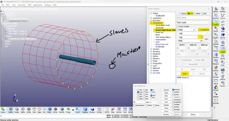
• Here the yellow web shows the CNRBs created for one portion of the inner cylinder. The center node is selected first followed by the other nodes at the periphery. This process is repeated with the other sides as well. Also, use this method to create CNRBs for the inner cylinder as well.
• 1007(red web),1009(blue web) for outer red cylinder & 1008(yellow web),1010(green web) for inner blue cylinder.

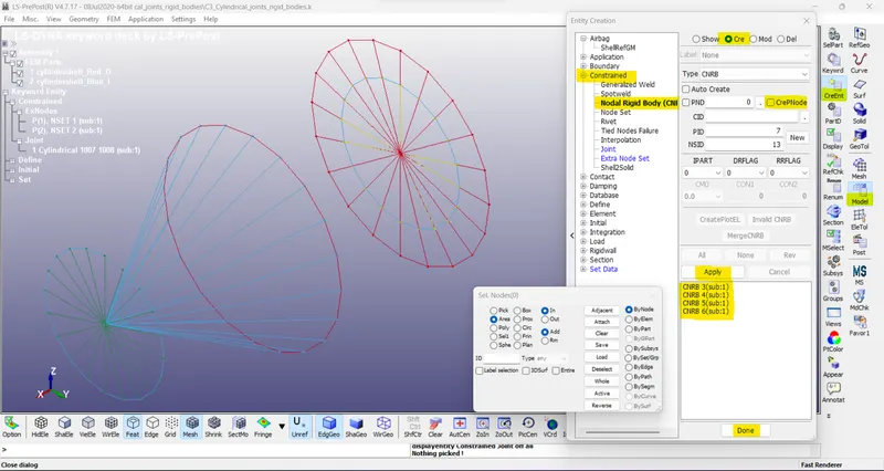
• For deformable bodies, the material is assigned using the *MAT_ELASTIC keyword. Here also the material card and section card are finally assigned to the part id.
• The cylindrical joint is defined by using the *CONSTRAINED_JOINT keyword. Four nodes should be defined to create a cylindrical joint. Here N1 and N3 belong to part A and N2 and N4 belong to part B.

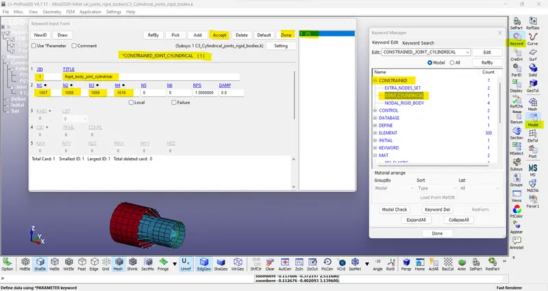
• Here also *CONSTRAINED_EXTRA_NODES should not be used.
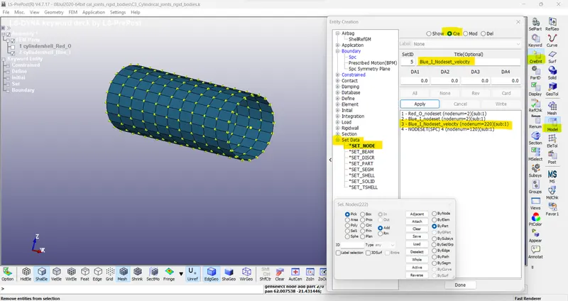
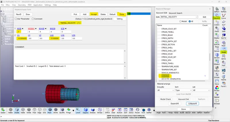
• Now an *INITIAL_VELOCITY card is created to assign the velocity. Before that, a node-set has to be created containing all the nodes from the inner blue cylinder. Since the cylindrical joint possesses both translational and rotational motion about a particular axis, we may assign it accordingly.
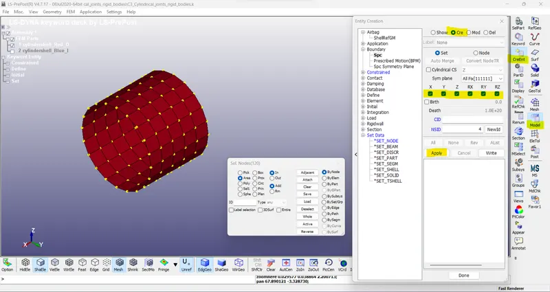
• Create Spc for the outer red cylinder fix from all DOFs.
• 
• 

Initial_Velocity-

Control-cards:

1. Control cards Such as Control Termination, And Control Time step Is Defined.
2. As INITIAL_VELOCITY_RIGID_BODY with a small run time is given Explicit Solver Is chosen for better results.

• Control Termination Card Is defined With the Termination Time 1ms.
• Database Binary D3Plot is defined to print the Results at 0.1ms in each interval.
• Control Timestep Card is defined For Stable Time Step.

• *CONTROL_TIMESTEP card is used and a load curve which is shown below is assigned through the LCTM option. The timestep calculated by the solver for these rigid bodies and this mesh size is large enough hence for more stability, we use smaller time steps for explicit analysis.

Post-processing:

Results:

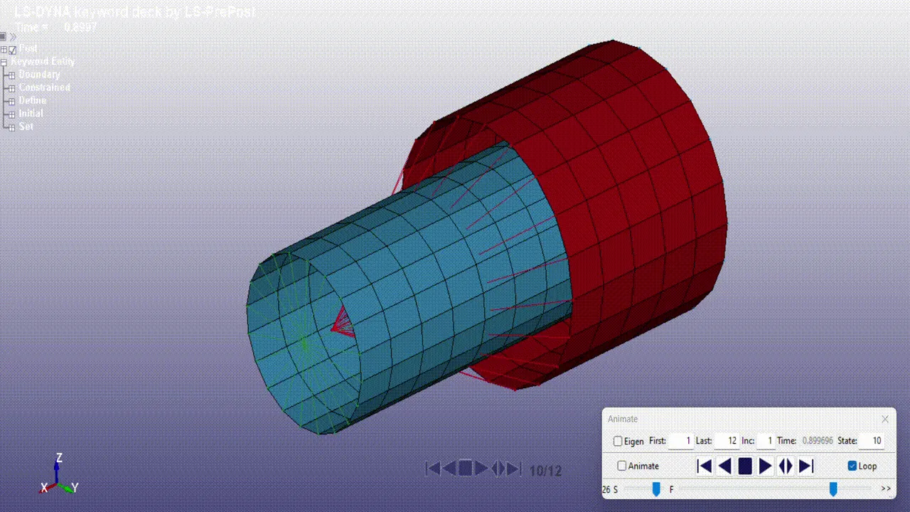
• The cylindrical joint between two deformable bodies using CNRBs is shown below.

The spherical joint:

/ Creating geometry for cylindrical joint -

• Two cylindrical shell elements (inner and outer) are created using the Element and mesh > Shape Mesher > Entity > Sphere shell option available in LS-PrePost.
• For representing the outer part few elements need to be deleted and it can be done using Element Tool > Node editing > Delete.

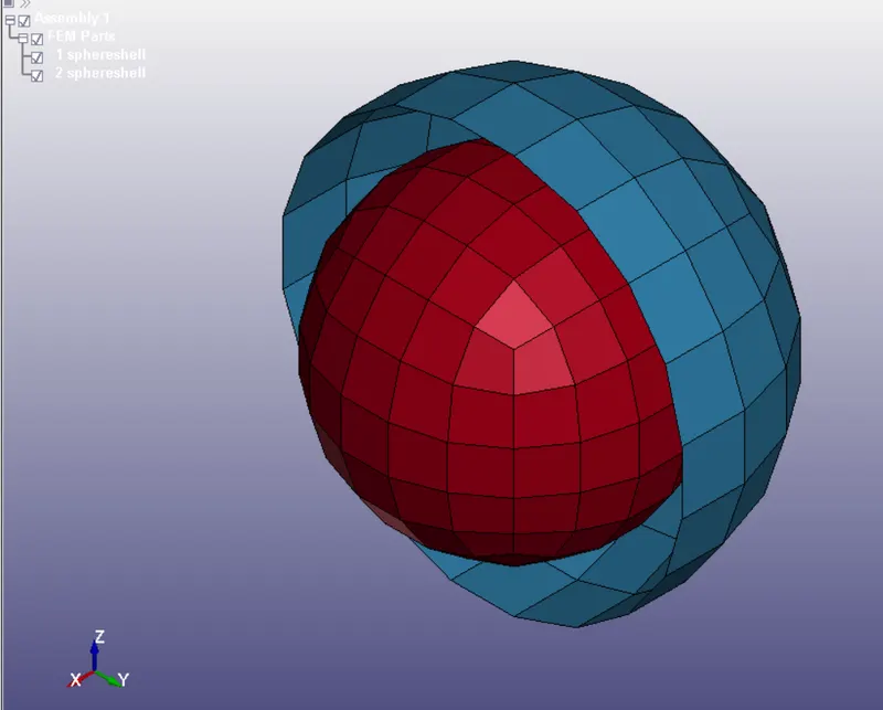
1. Spherical joint between two rigid bodies using *CONSTRAINED_EXTRA_NODES.

• Define a section property as a shell for created elements by using the *SECTION_SHELL keyword. Also, define a rigid material using the *MAT_RIGID keyboard. Use a reasonable value while defining the material properties. Define the respective MATID and SECID for the two parts.

• Create two extra nodes manually which are further needed to be associated with two parts for making a spherical joint. Create nodes by Element Tool > Node Editing option to give distinct node ids for all two nodes. From there use the 'by one' option to create the node at the center. (To make that two points in the center put x,y, and z coordinates as 0,0,0 at the origin)

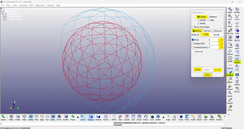
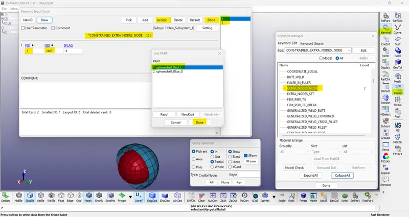
• These newly created nodes are in the space and do not belong to any of the parts now. So, for associating these nodes with part 1 and part 2, *CONSTRAINED_EXTRA_NODES_NODE is used.

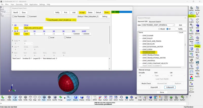
• Now, the spherical joint is defined by using the *CONSTRAINED_JOINT keyword. The two nodes should be defined to create a spherical joint. N1 belongs to body 1 and N2 belongs to body 2.

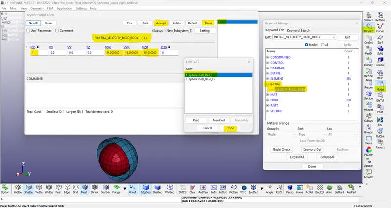
• Now an *INITIAL_VELOCITY_RIGID_BODY card is created to assign the velocity by selecting the required PID.

Control-cards:

1. Control cards Such as Control Termination, And Control Time step Is Defined.
2. As INITIAL_VELOCITY_RIGID_BODY with a small run time is given Explicit Solver Is chosen for better results.

• Control Termination Card Is defined With the Termination Time 1ms.
• Database Binary D3Plot is defined to print the Results at 0.1ms in each interval.
• Control Timestep Card is defined For Stable Time Step.

• *CONTROL_TIMESTEP card is used and a load curve which is shown below is assigned through the LCTM option. The timestep calculated by the solver for these rigid bodies and this mesh size is large enough hence for more stability, we use smaller time steps for explicit analysis.

Post-processing:

Results:

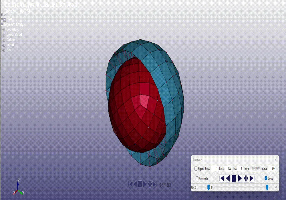
• The spherical joint between two rigid bodies using *CONSTRAINED_EXTRA_NODES is shown below.

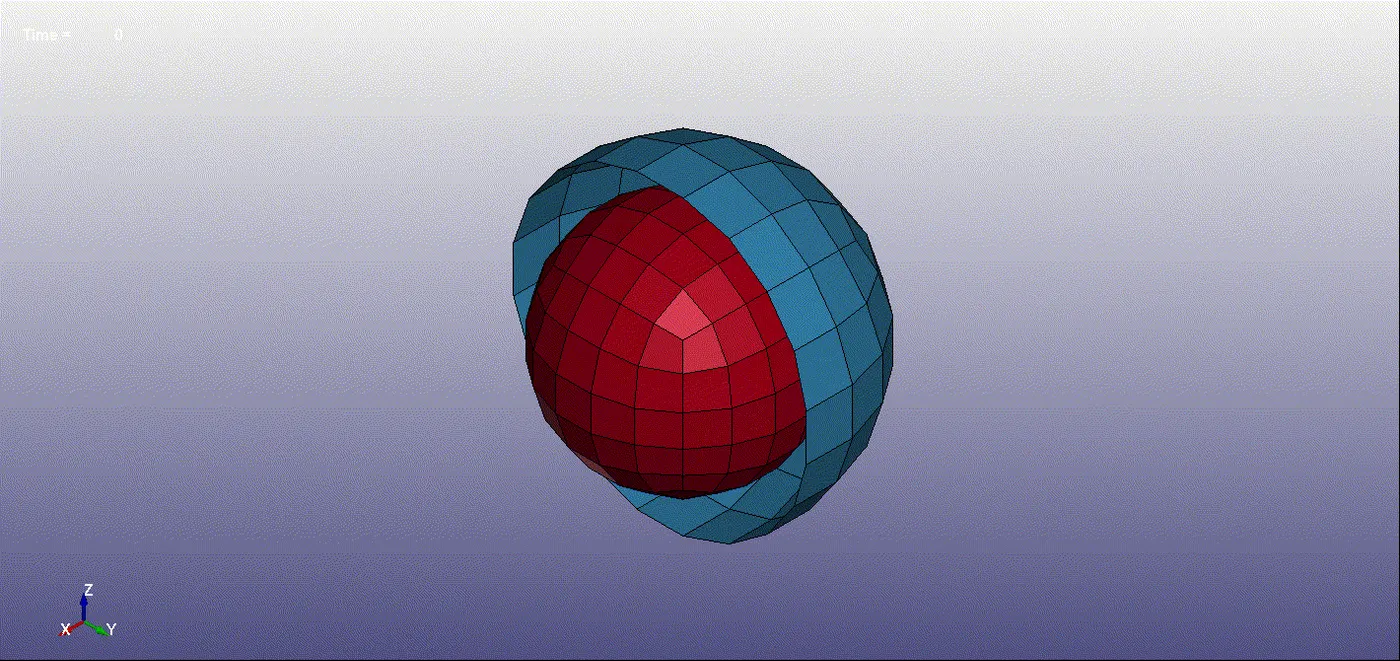
2. The spherical joint between two deformable bodies using CNRBs

• The spherical joint between two deformable joints is created with the help of *CONSTRAINED_NODAL_RIGID_BODY(CNRB).

• At first, four nodes are created which would be further used to create CNRBs. Create nodes by Element > Tools > Node Editing and give distinct node IDs for all two nodes.

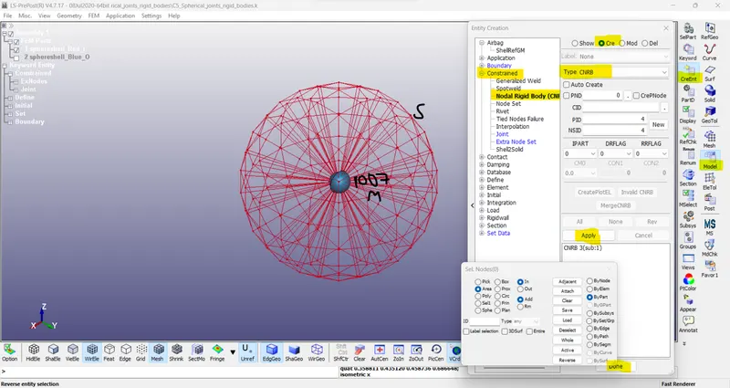
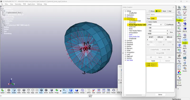
• To create a CNRB, go to Create Entity > Constrained > Nodal Rigid Body (CNRB) > Create. Toggle off the CrePNode option which will disable the creation of PNODE at the mass center of the selected nodes.

• First, take any part (inner or outer), select the middle node, and then other nodes as did with the cylindrical joint.

• For deformable bodies, the material is assigned using the *MAT_ELASTIC keyword. Here also the material card and section card are finally assigned to the part id.

• The spherical joint is defined by using the *CONSTRAINED_JOINT keyword. The two nodes should be defined to create a spherical joint. Here N1 belongs to part A and N2 belongs to part B.

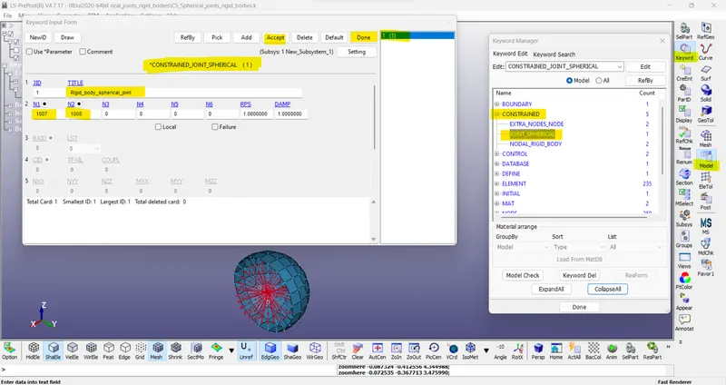
• Here also *CONSTRAINED_EXTRA_NODES should not be used.

• Now an *INITIAL_VELOCITY card is created to assign the velocity. Before that, a node-set has to be created containing all the nodes from the inner Red sphere.
• Create Spc for the outer Blue sphere fix from all DOFs.

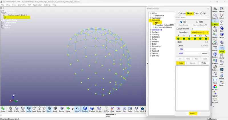
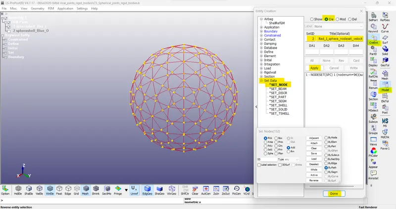
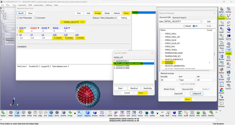
• *CONTROL_TIMESTEP card is used and a load curve is assigned similar to that of the models done above.
• Other required post-processing cards are assigned and then it's been run in the Ls-program manager.

Post-processing:

Results:

• The spherical joint between two deformable bodies using *CONSTRAINED_NODAL_RIGID_BODY (CNRB) is shown below.

The translational joint:

/ Creating geometry for translational joint-

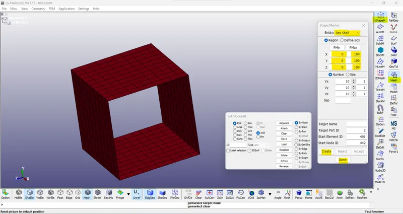
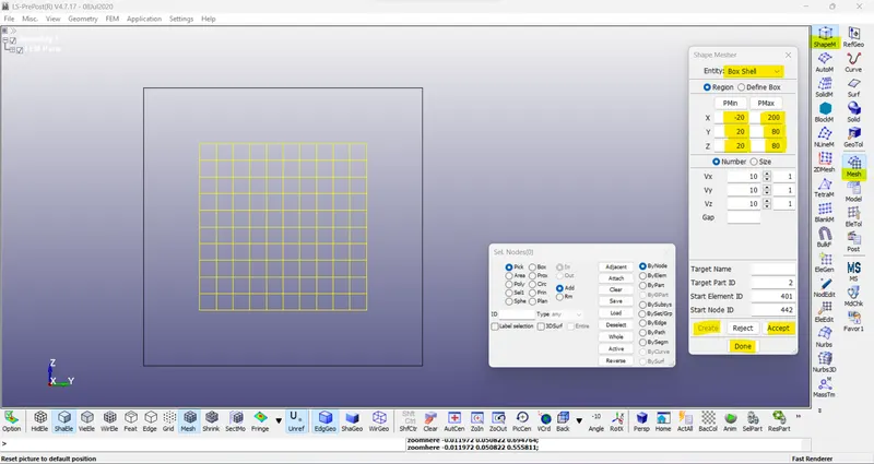
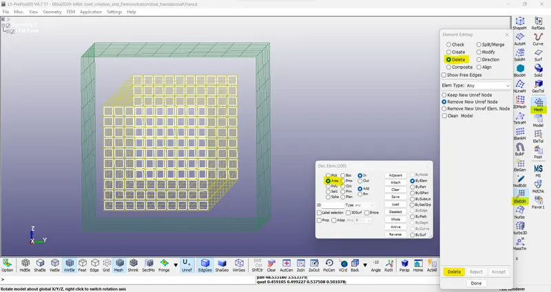
• A Box Shell is created first using the Mesh > Shape Mesher > Entity > Box Shell option. After that, two faces along the X-axis of box elements are deleted from Mesh > Element edit > delete. After creating 1 box, create the other box similarly with appropriate coordinates.

1. Translational joint between two rigid bodies using *CONSTRAINED_EXTRA_NODES.

• Define a section property as a shell for created elements by using the *SECTION_SHELL keyword. Also, define a rigid material using the *MAT_RIGID keyboard. Use a reasonable value while defining the material properties. Define the respective MATID and SECID for the two parts.

• Create six extra nodes manually which are further needed to be associated with two parts for making a translational joint. Create nodes by Element Tool > Node Editing option to give distinct node ids for all six nodes. From there use the 'by two' option to create the node at the center. Here three pair of nodes is defined. The third pair of nodes is defined in between the other two pairs and slightly displaced from the axis of the other two pairs.

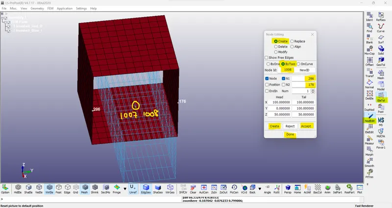
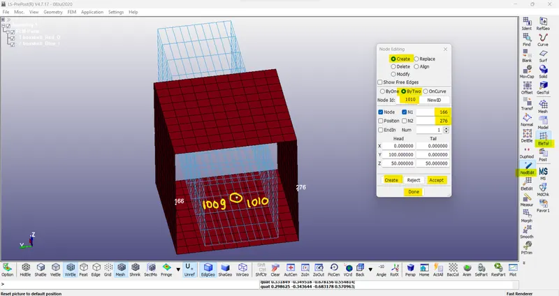
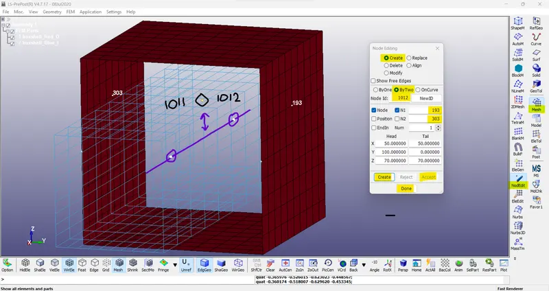
/Note- create node-set for these newly created nodes 1007,1009,1011 for the Red outer box & 1008,1010,1012 for the Blue inner box.

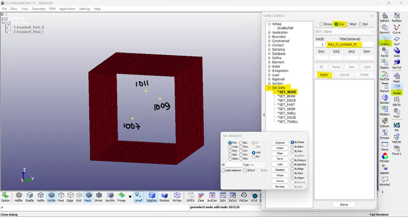
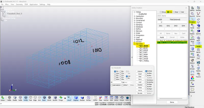
• These newly created nodes are in the space and do not belong to any of the parts now. So, for associating these nodes with part 1 and part 2, *CONSTRAINED_EXTRA_NODES_SET is used.

• Now, the translational joint is defined by using the *CONSTRAINED_JOINT keyword. Six nodes should be defined to create a translational joint. (N1, N3, N5) belong to body 1 and (N2, N4, N6) belong to body 2.

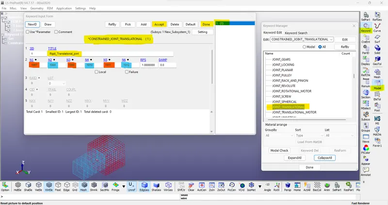
• A displacement curve was also defined for the prescribed motion keyboard which is defined by LCID.

• After that, the curve is assigned to the *PRISCRIBED_MOTION_RIGID card.

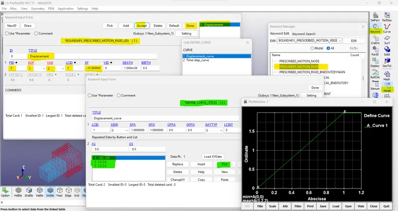
• *CONTROL_TIMESTEP card is used and a load curve is assigned similar to that of the models done above.
• Other required post-processing cards are assigned and then it's been run in the Ls-program manager.

Post-processing:

Results:

• The translational joint between two rigid bodies using *CONSTRAINED_EXTRA_NODES is shown below.

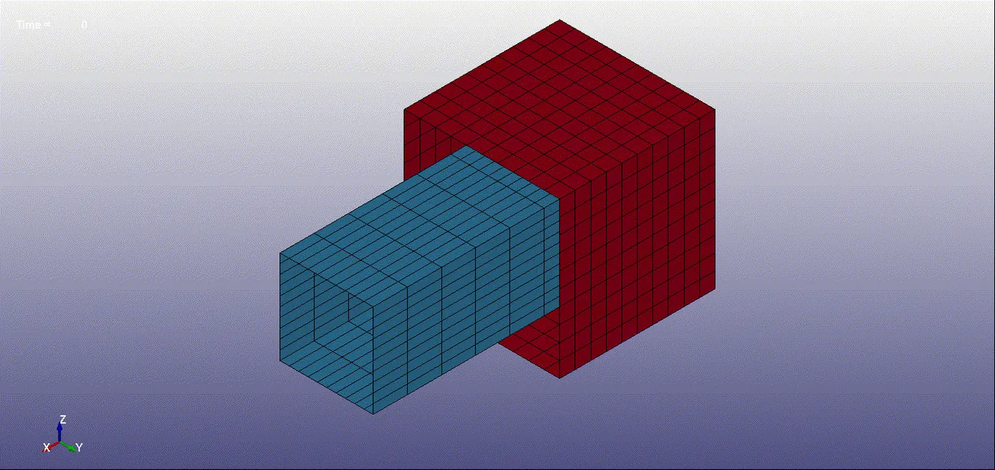
2. The translational joint between two deformable bodies using CNRBs

• Here the translational joints between two deformable bodies are created with the help of *CONSTRAINED_NODAL_RIGID_BODY(CNRB).

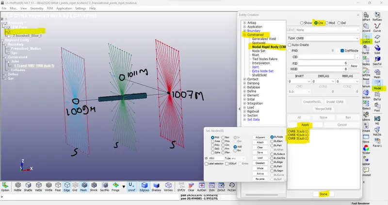
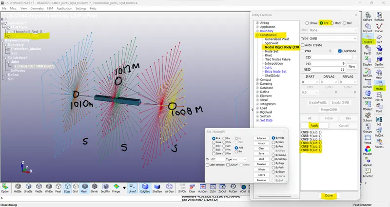
• At first, six nodes are created which would be further used to create CNRBs. Create nodes by Element > Tools > Node Editing and give distinct node IDs for all six nodes.

• To create a CNRB, go to Create Entity > Constrained > Nodal Rigid Body (CNRB) > Create. Toggle off the CrePNode option which will disable the creation of PNODE at the mass center of the selected nodes.

• First, take any part (inner or outer), select the middle master node first, and then other slave nodes as did with the other bodies (cylindrical) above.

• For deformable bodies, the material is assigned using the *MAT_ELASTIC keyword. Here also the material card and section card are finally assigned to the part id.

• Now, the translational joint is defined by using the *CONSTRAINED_JOINT keyword. Six nodes should be defined to create a translational joint. (N1, N3, N5) belong to body 1 and (N2, N4, N6) belong to body 2.

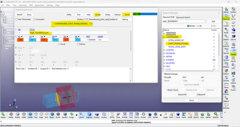
• Here also *CONSTRAINED_EXTRA_NODES should not be used.
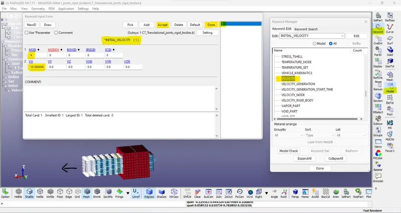
• The velocity is defined using the *INITAL_VELLOCITY card. Before that, a node-set should be created which includes all the nodes of the moving Blue inner part.
• Also, an Spc set with all DOFs fixed for the Red outer part.

Post-processing:

Results:

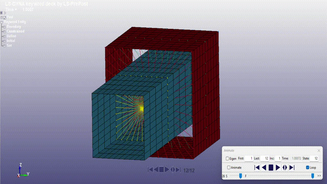
• The translational joint between two deformable bodies using CNRBs is shown below.

Conclusion:

• The joint demonstration for revolute, cylindrical, spherical, and translational joints between two rigid bodies also with two deformable bodies using the *CONSTRAINED_JOINT keyword is done successfully. Here we have used *CONSTRAINED_EXTRA_NODES and CNRBs to create the joint accordingly for two cases. Although the definition of joints for the two cases remains the same, the ways of implementation differ.