Week 8 - Simulating Cyclone separator with Discrete Phase Modelling

Aim- To perform analysis on cyclone separator and calculate the separation efficiency and pressure drop.

Introduction- A cyclone separator is simply a separation device used for gas-solid flow. This flow needs to be filtered from the particulate matter. The principle on which this device works is simply inertia, where the gas having lower inertia gets separated from the solid particles having higher inertia due to its weight and density. Cyclone separators are genrally used as a pollution control device called as precleaners. It is mainly used in industried where flue gases are liberated in air, which calls in the need of a filter to filter the air as clean as it can be to avoid air pollution and not jeopardize the pollution norms of the government. The size of this device can vary depending on the amount of flue gases filtered, thus larger operations tend to require larger seperators. For example, several different models of the same cyclone separator can exist, and the size can range from a relatively small 1.2-1.5 meters tall (4-5 feet) to around 9 meters (30 feet) which is around the height of a 3 storey building.

Theory-

Working principle-

Cyclone separators work much like a centrifuge, but with a continuous feed of dirty air. In a cyclone separator, dirty flue gas is fed into a chamber. The inside of the chamber creates a spiral vortex, similar to a tornado. This spiral formation and the separation is shown in the figure below. The lighter components of this gas have less inertia, so it is easier for them to be influenced by the vortex and travel up it. Contrarily, larger components of particulate matter have more inertia and are not as easily influenced by the vortex.

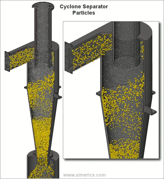
Since these larger particles have difficulty following the high-speed spiral motion of the gas and the vortex, the particles hit the inside walls of the container and drop down into a collection hopper. These chambers are shaped like an upside-down cone to promote the collection of these particles at the bottom of the container. The cleaned flue gas escapes out the top of the chamber.

Empirical models for Cyclone separator efficiency-

• Iozia and Leith model-

Iozia and Leith (1990) logistic model is a modified version of Barth (1956) model which is developed based on force balance. The model assumes that a particle carried by the vortex endures the influence of two forces: a centrifugal force, Z, and a flow resistance, W. Core length, zc, and core diameter, dc.

The addition made by Iozia and Leith on the original Barth (1956) model are the core length zc and slope parameter β expression which is derived based on the statistical analysis of experimental data of cyclone with D = 0.25 m.

• Li and Wang model-

The Li and Wang (1989) model includes particle bounce or re-entrainment and turbulent diffusion at the cyclone wall. A two-dimensional analytical expression of particle distribution in the cyclone is obtained. Li and Wang model was developed based on the following assumptions:
• The radial particle velocity and the radial concentration profile are not constant, for uncollected particles within the cyclones.
• Boundary conditions with the consideration of turbulent diffusion coefficient and particle bounce re-entrainment on the cyclone wall are:

c = c0, at θ = 0

• Koch Licht model-

Koch and Licht (1977) collection theory recognized the inherently turbulent nature of cyclones and the distribution of gas residence times within the cyclone. Koch and Licht describe particle motion in the entry and collection regions with the additional following assumptions:
• The tangential velocity of a particle is equal to the tangential velocity of the gas flow, i.e. there is no slip in the tangential direction between the particle and the gas.
• The tangential velocity is related to the radius of cyclone by: uRn = constant

• Lapple model-

Lapple (1951) model was developed based on force balancewithout considering the flow resistance. Lapple assumed that a particle entering the cyclone is evenly distributed across the inlet opening. The particle that travels from inlet half width to the wall in the cyclone is collected with 50% efficiency.

Solving and Modelling approach-

Lets discuss about the methods available for performing this simulation.

Types of phases for a flow-

• Continuous phase
• Discrete phase

Continuous phase-

It consists of fluid flowing within the fluid volume.

Discrete phase-

It consists of fine solid particles with the continuous phase.

It can also exchange momentum, mass and energy with Fluid phase or Continuous phase.

To use this kind of phase in our solution DPM(Discrete Phase Modelling) is used in the solver setting.

Discrete Phase Modelling-

It is enabled when there are solid particles in gas, liquid or liquid droplets in gas or bubbles in liquid.

There are two ways to carry out DPM-

• Coupled flow
• Uncoupled flow

Coupled flow-

The discrete phase influences the flow of continuous phase.

Uncoupled flow-

In this type of flow the discrete phase does not interact with the continuous phase.

Since the size of the particulate injected is very fine the use of either of the methods would not matter much.

Analysis approach-

• Case I - Varying the particle diameter.
• Case II - Varying the particle velocities.

Formulae-

1. Separation efficiency = Number of particles trapped / Number of particles tracked
2. Pressure drop = Inlet pressure - outlet pressure

Pre-processing and solver setting-

Geometry-

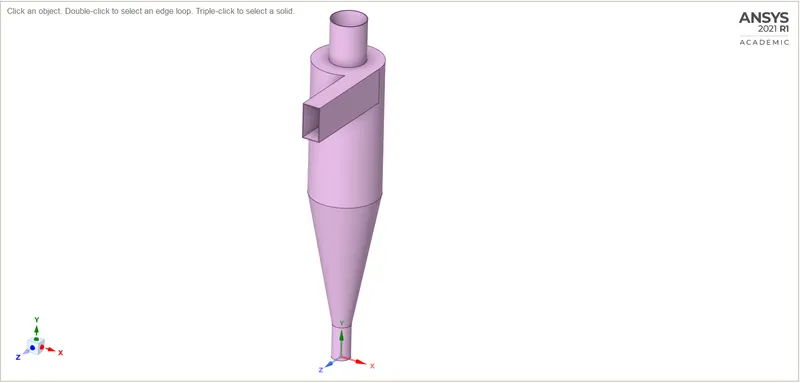
Model before volume extraction-

Model after volume extraction-

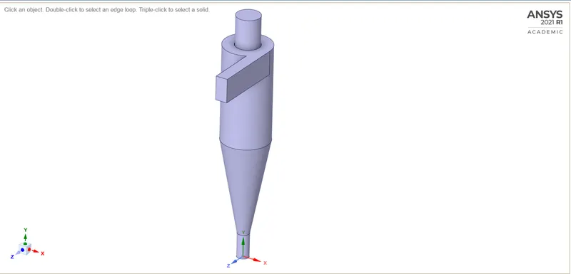
The body is suppressed for physics and fluid volume is enabled and taken further for solving.

Meshing-

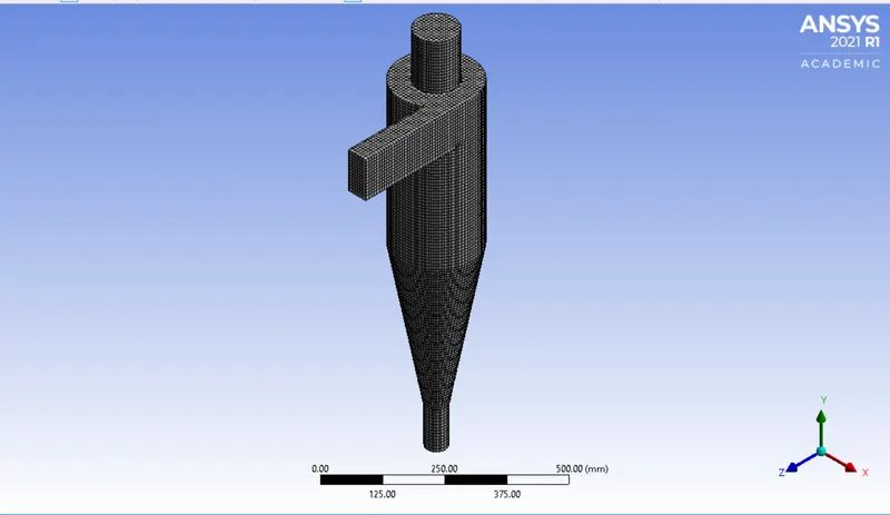
Element size = 10mm

Number of elements = 52613

Body sizing = 6mm

Body fitted cartesian = default size

Named selections = inlet, outlet1(top), outlet2(bottom/dustbin)

Fluent-

Steps for Fluent solver -

1. Perform Mesh check
2. Select the steady state solver
3. Enable gravity in the negative y-direction as -9.81m/s^2
4. Select the k-epsilon viscous model and select RNG, swirl dominated options in the same window.
5. Click on Discrete phase model, check the interaction with continuous phase, update DPM sources, DPM interaction interval (keep default value as 10).
6. In the same window click Injections below, create one and check on inert, select anthracite as the solid particle, select surface injection as the type of injection, select inlet as the source of injection and give the X-velocity your value of magnitude of velocity which acts normal to the surface selected. Give the diameter of the solid particle (between 1e-6 and 5e-6) in microns.
7. Give the Boundary conditions. Velocity magnitude of inlet with respect to the case.
8. In boundary conditions select DPM and give the discrete phase BC type to every named selection. The discrete phase BC types for inlet and wall is reflect, for outlet(top) is escape, for outlet(bottom/dustbin) is trap.
9. Open Methods in Solution and change the Turbulent Kinetic energy and Turbulent Dissipation rate as Second order upwind.
10. Initialize the solution using standard method by computing it from inlet.
11. Hit calculate for 600 iterations.
12. After the solution is ready extract the particle history by selecting export from file in the left top corner move the cursor over export and select particle history data. Select the injection created from step (6), click browse and save the file. Click write and note down the number of particle trapped, tracked, escaped and incomplete.

CFD Post-processing-

1. Display the wall component. Render it to be transparent
2. Click File and import the particle history data by browsing the saved file.
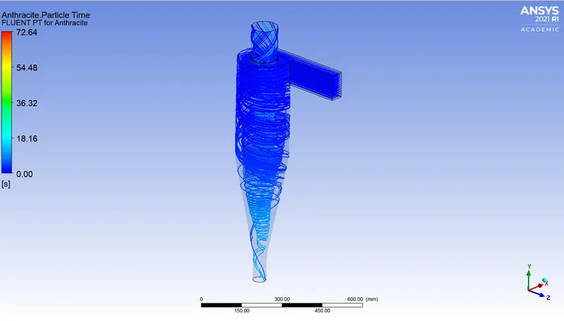
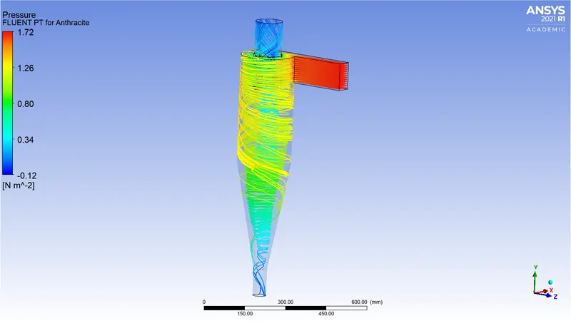
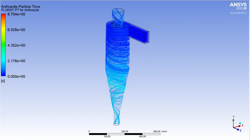
3. Colour the particle with variables to have visuals over various parameters, such as Residence time, pressure as in this report.

Case I - Varying particle diameter

• Particle diameter = 1um

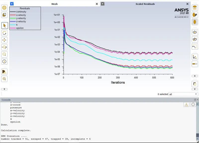
Separation efficiency = (39/91)x100 = 42.85%

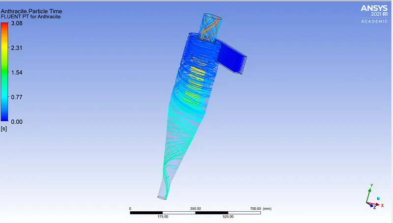
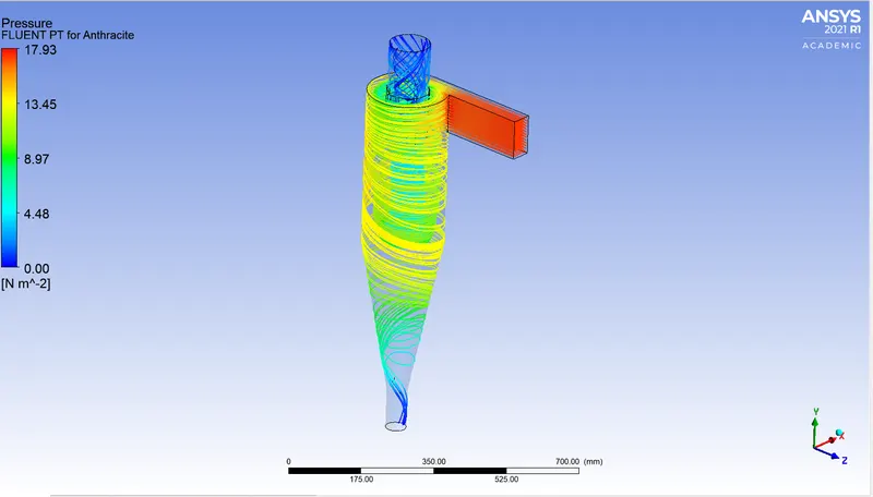
• Particle diameter = 2um

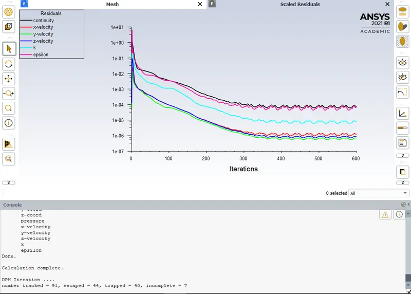
Separation efficiency = (40/91)x100 = 43.95%

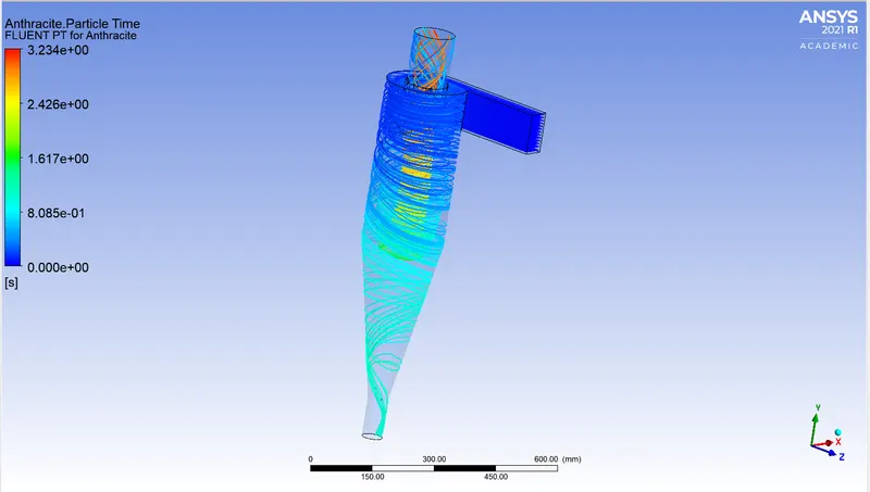
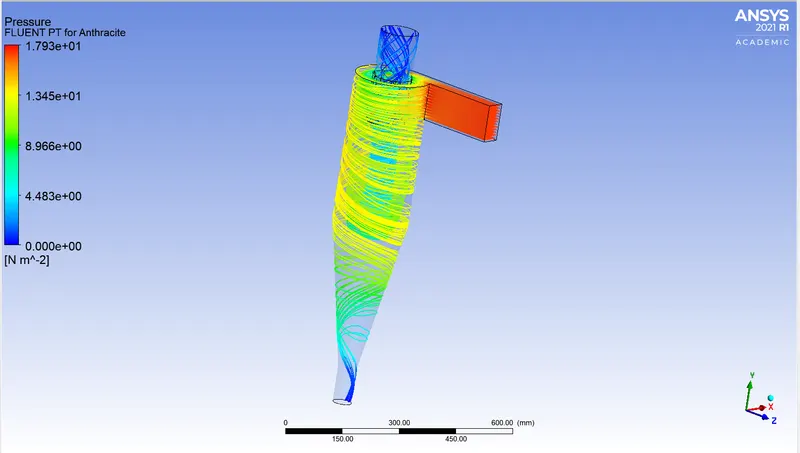
• Particle diameter = 3um

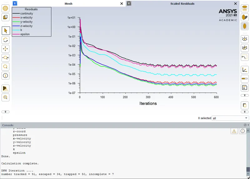
Separation efficiency = (50/91)x100 = 54.94%

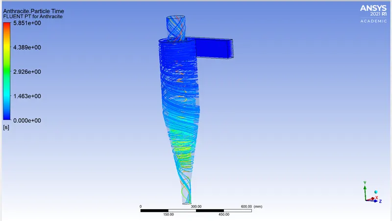
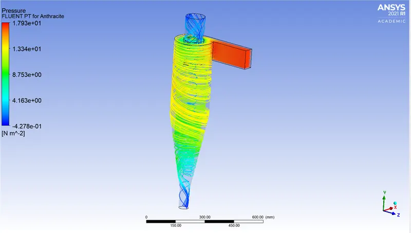
• Particle diameter = 4um

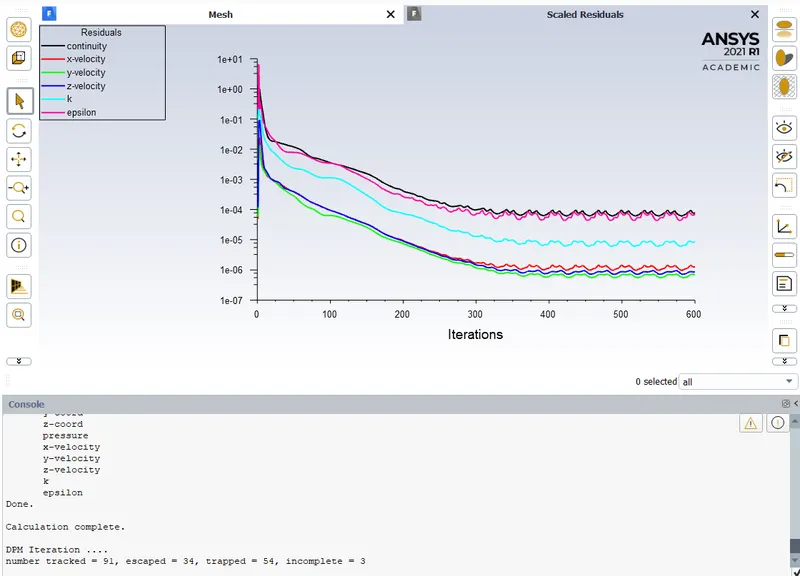
Separation efficiency = (54/91)x100 = 59.34%

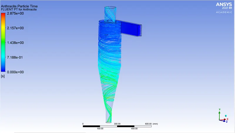
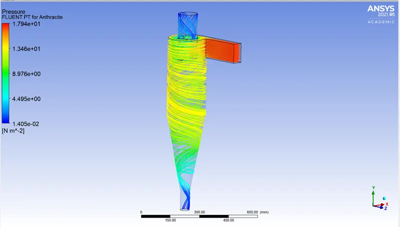
• Particle diameter = 5um

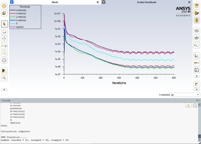
Separation efficiency = (56/91)x100 = 61.53%

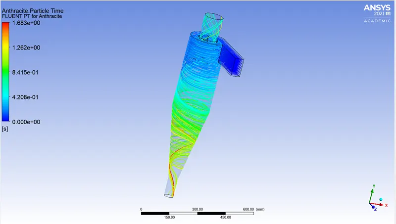
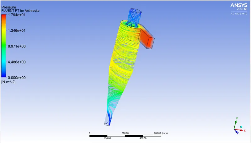
Case II - Varying particle velocity-

• Particle velocity = 1m/s

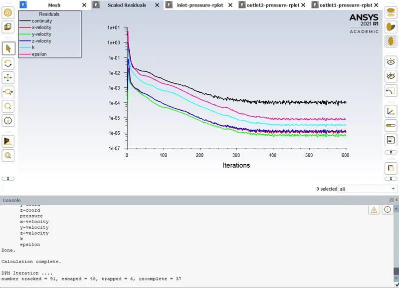
Separation efficiency = (6/91)x100 = 6.59%

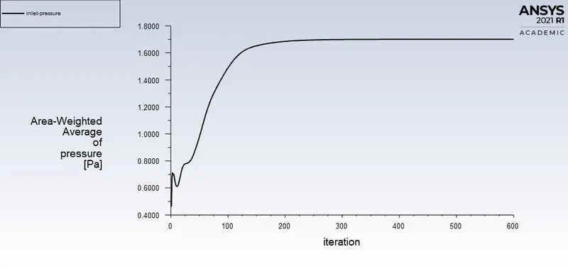
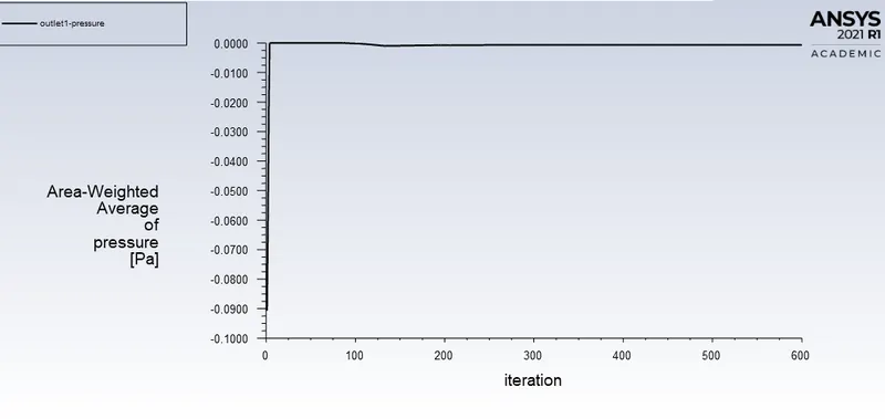
Pressure drop = 1.7Pa - 0Pa = 1.7Pa

• Particle velocity = 2m/s

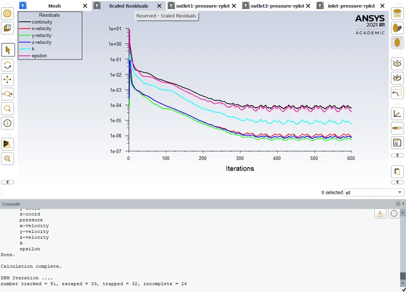
Separation efficiency = (32/91)x100 = 35.16%

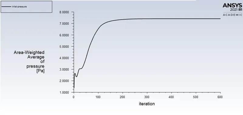
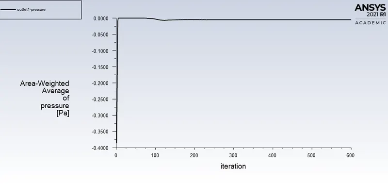
Pressure drop = 7.25-(-0.0125) =7.2625Pa

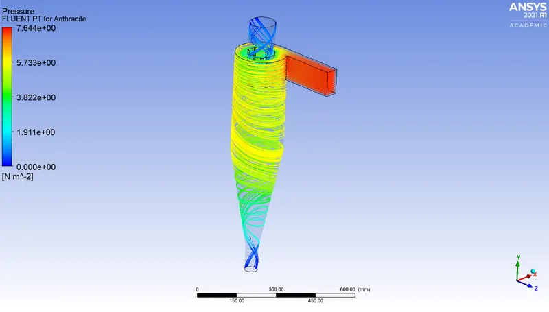
• Particle velocity = 3m/s

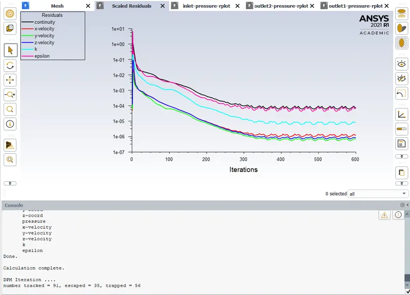
Separation efficiency = (56/91)x100 = 61.53%

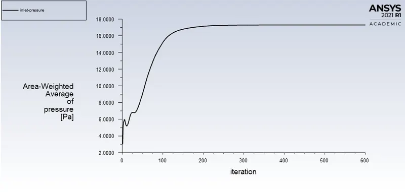
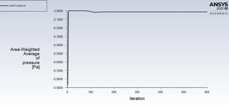
Pressure drop = 17-(-0.025) = 17.025Pa

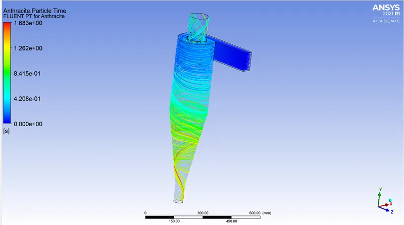
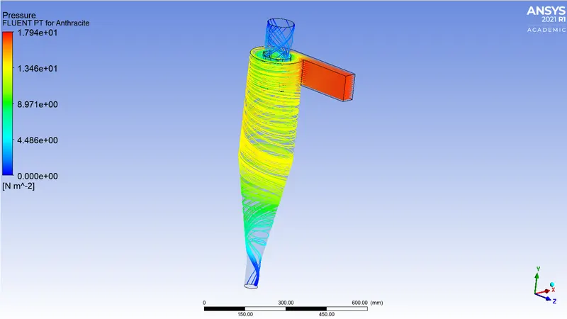
• Particle velocity = 4m/s

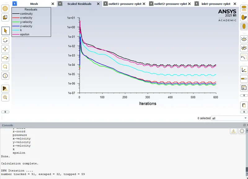
Separation effciency = (59/91)x100 = 64.83%

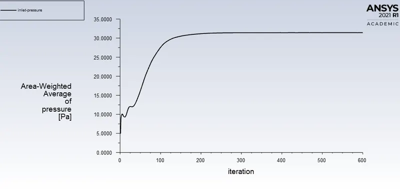
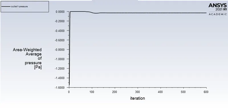
Pressure drop = 30-(-0.1) = 30.1Pa

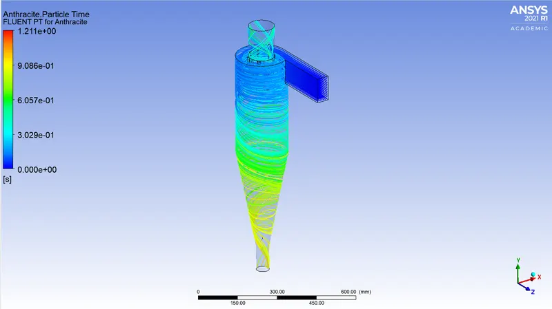
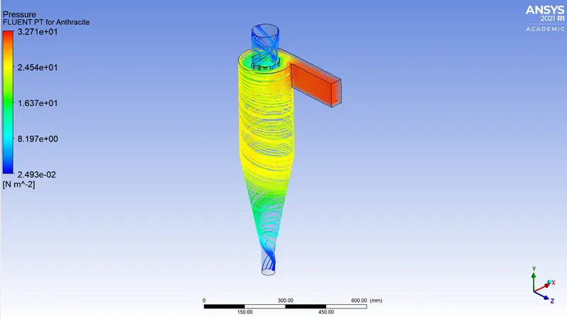
• Particle velocity = 5m/s

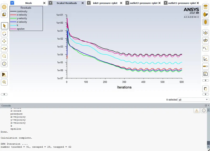
Separation efficiency = (62/91)x100 = 68.13%

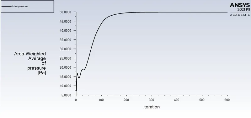
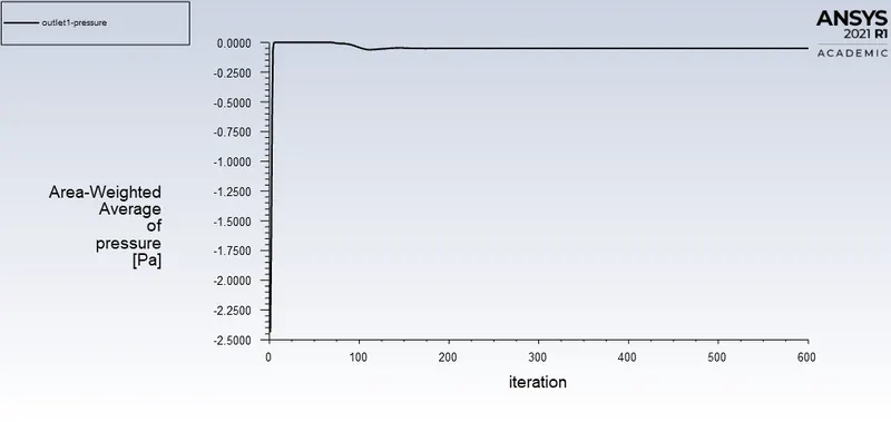
Pressure drop = 47.75-(-0.1) = 47.85Pa

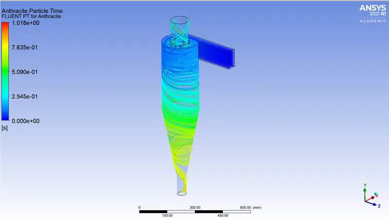
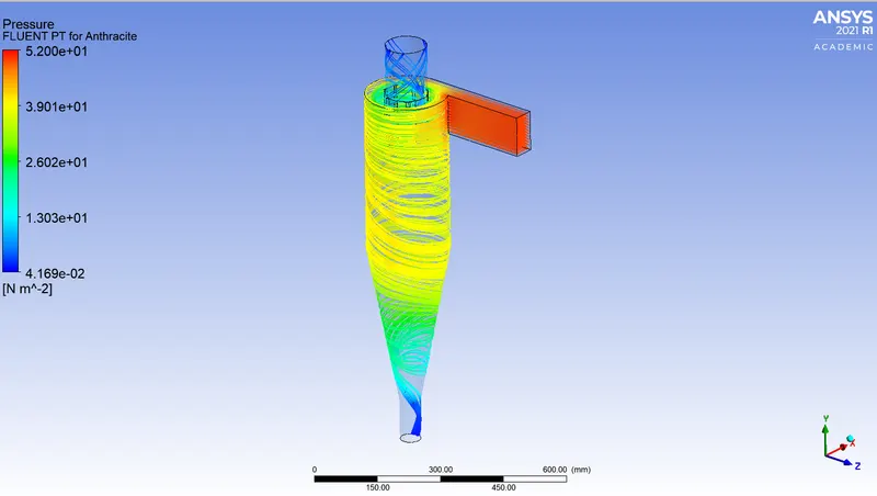
Table for Case I -

Particle diameter	Particle velocity	Particle tracked	Particle trapped	Separation efficiency
1μm	3m/s	91	39	42.85%
2μm	3m/s	91	40	43.95%
3μm	3m/s	91	50	54.94%
4μm	3m/s	91	54	59.34%
5μm	3m/s	91	56	61.53%

Table for Case II -

Particle diameter	Particle velocity	Particle tracked	Particle trapped	Separation efficiency	Pressure drop
5μm	1m/s	91	6	6.59%	1.7 Pa
5μm	2m/s	91	36	35.16%	7.2625 Pa
5μm	3m/s	91	56	61.53%	17.025 Pa
5μm	4m/s	91	59	64.83%	30.1 Pa
5μm	5m/s	91	62	68.13%	47.85 Pa

Conclusion-

• For Case I, as the particle diameter increases, the separation efficiency increases which means the number of particles trapped increases in the bottom outlet or the dustbin. This is because of the increases inertia of the particle due to its increases in size.
• For Case II, as the particle velocity is increased with the flow velocity the separation efficciency increases, the higher velocity helps the particle to travel faster which reduces the inertia of the particle and allows it to settle down in the dustbin.
• It is observed that for the first 3 setting of Case I and Case II there exist a number of particles which are incomplete, which prompts that at low velocity and smaller particle diameter the travel takes longer than 600 iterations for it to either get trapped in the dustbin or escape through the top outlet.
• The pressure drop increases with the increase in velocity, the reason behind being increase in the inlet pressure due to increase in the flow velocity.