Project 1 - Parsing NASA thermodynamic data

Aim -

1. To write a function that extracts the 14 co-efficients and calculates the enthalpy, entropy and specific heats for all the species in the data file.

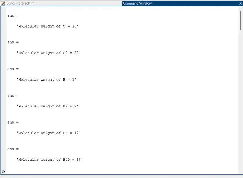
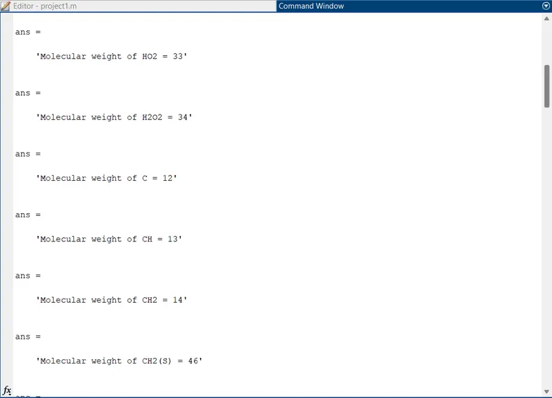
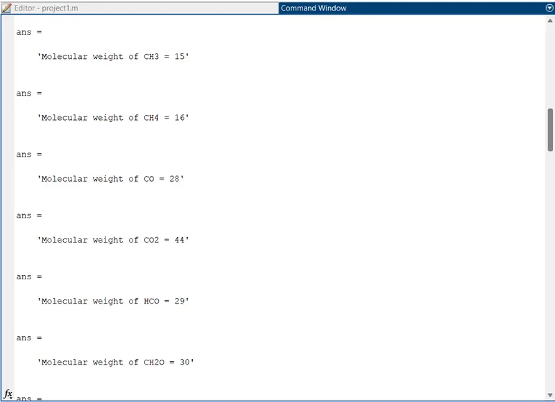
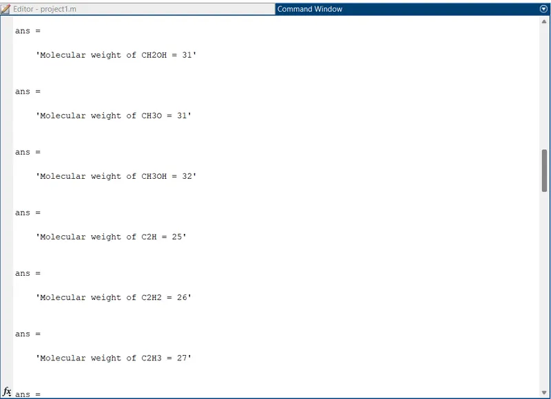
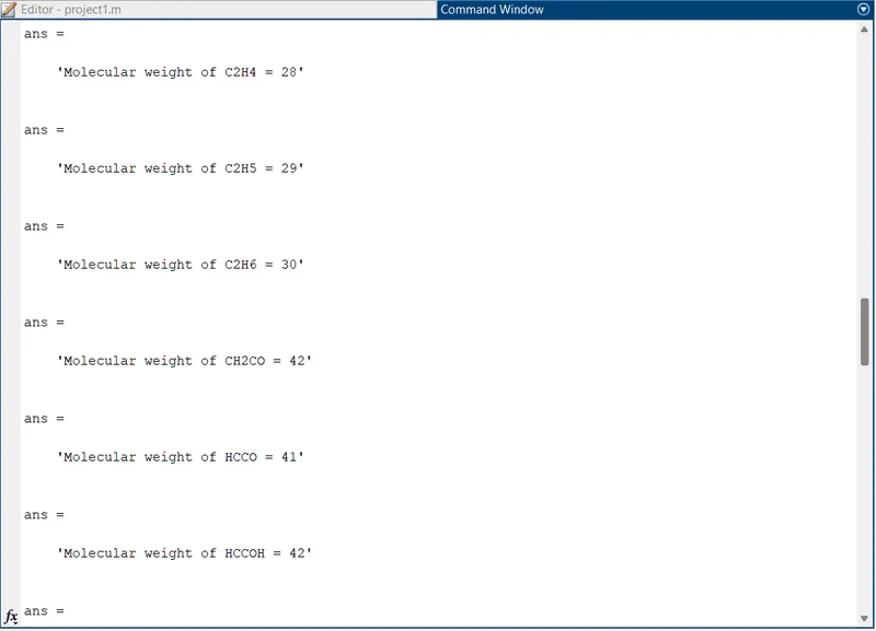
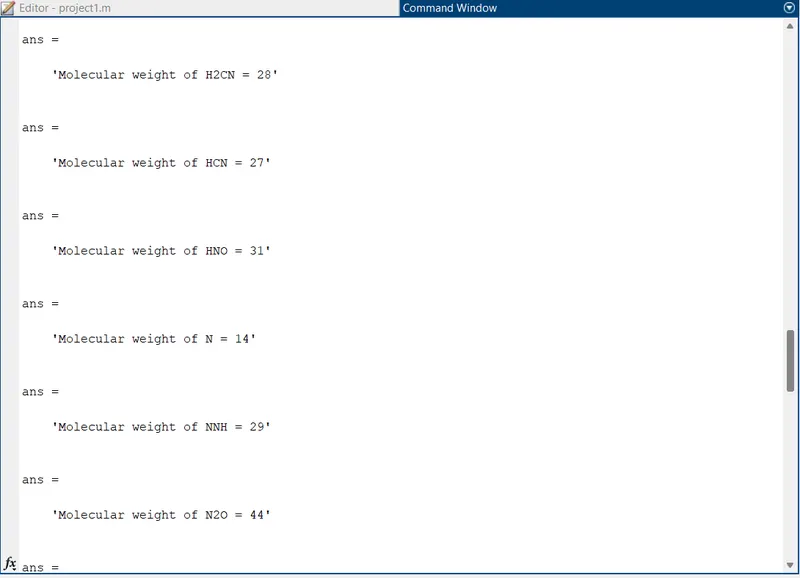
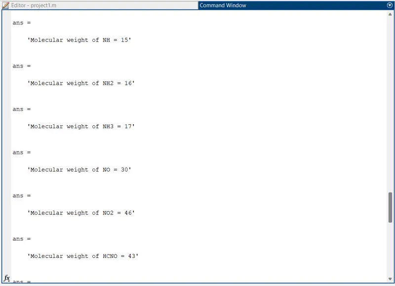
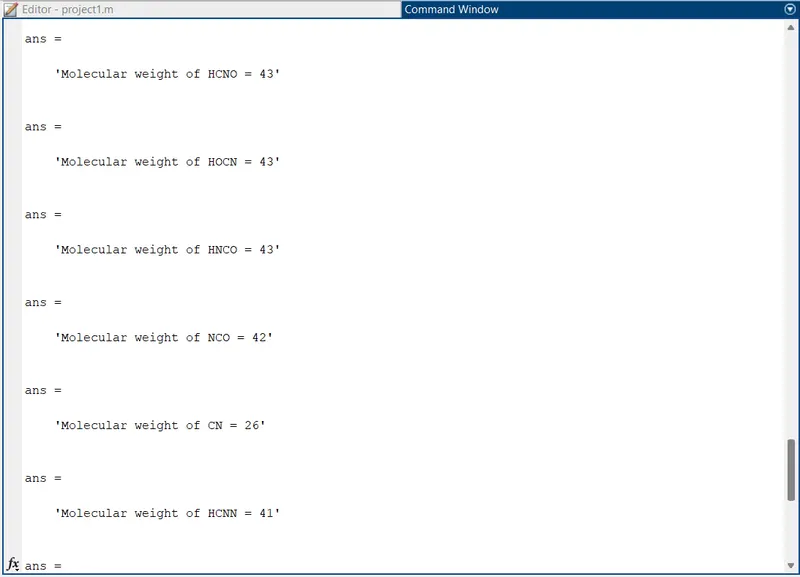
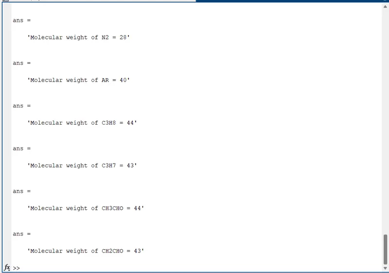
2. Calculate the molecular weight of each species and display it in the command window.

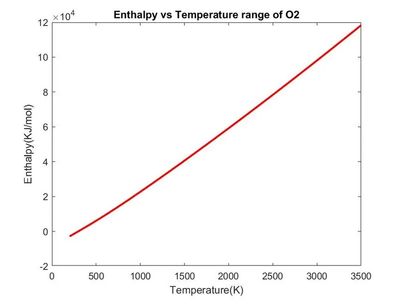
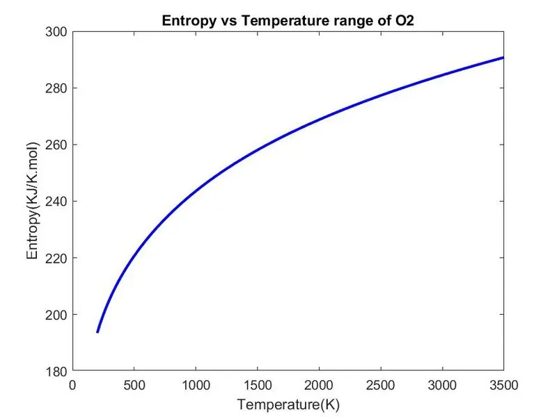
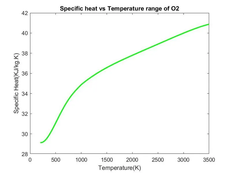
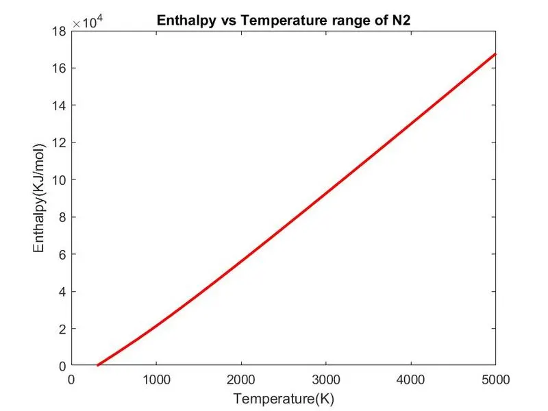
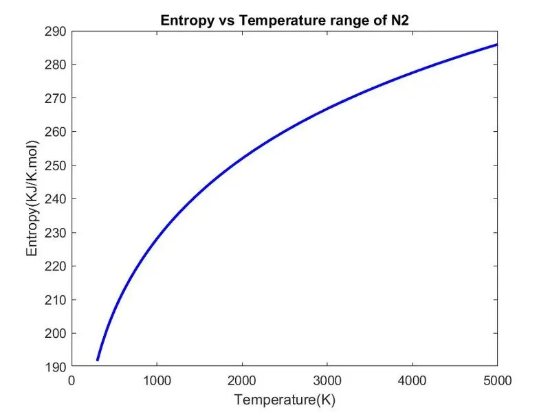
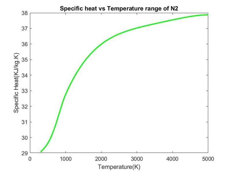
3. Plot the Cp, Enthalpy and Entropy for the local temperature range (low temperature : high temperature) specific for each species.

4. Save the plots as images with appropriate names and dump them in separate folders for each species with suitable name.

Introduction & Theory-

Data parsing is the process of taking data in one format and transforming it to another format. Data parsing is a method where one string of data gets converted into a different type of data. Parsing splits a file or other input into pieces that can be easily accessed and manipulated.

The NASA thermodynamic file -

This file contains the coefficients of 53 species which can be used to evaluate certain properties of the respective species such as the specific heat, enthalpy, entropy, etc. Alongwith the coefficients are given the temperature ranges within which the species react. With this information given in the .dat file we need to calculate the asked properties by parsing the required data from it and use the formulas all of which has to be coded using Matlab.

Formulas -

1. Specific Heat -

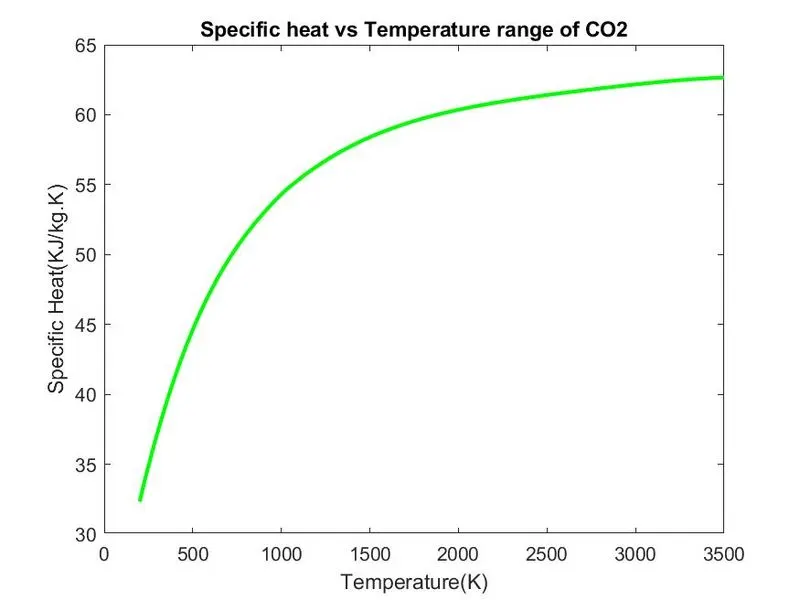
Cp = R*(a1 + (a2*T) + (a3*(T).^2) + (a4*(T).^3) + (a5*(T).^4))

The specific heat capacity of a substance is the heat capacity of a sample of the substance divided by the mass of the sample. Specific heat is also sometimes referred to as massic heat capacity.

Water has a specific heat capacity of 4.186 J/g°C, meaning that it requires 4.186 J of energy (1 calorie) to heat a gram by one degree. is the change in temperature of the system.

In engineering calculations the unit is often used as KJ/kg.K.

2. Enthalpy -

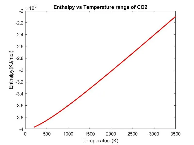
H = R*T.*(a1 + ((a2*T)/2) + ((a3*(T).^2)/3) + ((a4*(T).^3)/4) + ((a5*(T).^4)/5) + ((a6./T)))

Enthalpy, a property of a thermodynamic system, is the sum of the system's internal energy and the product of its pressure and volume. It is a state function used in many measurements in chemical, biological, and physical systems at a constant pressure, which is conveniently provided by the large ambient atmosphere.

Unit for enthalpy is given by energy per mass, i.e. KJ/kg.

3. Entropy -

Code-

1. Main code

clear all 
close all
clc

%Reading data 
f1 = fopen('THERMO.dat','r');
get = fgetl(f1);

%Reading temperature file from data
temp = fgetl(f1);

%splitting the temp values
s = strsplit(temp);

%Converting characters into numbers
temp_low = str2double(s{2});
temp_mid = str2double(s{3});
temp_high = str2double(s{4});

%Defining temperature range
%T = linspace(temp_low,temp_high,1000);

R=8.314;

% Skipping (2) + (3) comment lines
for  i = 1:3
    get = fgetl(f1);
end

%Reading species 
for j=1:53
    sp_line = fgetl(f1);
    A = strsplit(sp_line, ' ');
    species = (A{1});

    %Converting string to numbers 
    templow = str2double(A{end-3});
    tempmid = str2double(A{end-1});
    temphigh = str2double(A{end-2});
    T = linspace(templow,temphigh,1000);

    %moving to the next line of coefficeints and finding the string E among
    %them
    sp_line1 =  fgetl(f1);
    a = strfind(sp_line1, 'E');

    %Extracting the first 7 higher coefficients and the next 7 lower coeffs
    % The first 2 lines have 5 coeffs each 
    % HIGHER COEFFS -
    a1 = sp_line1(1:a(1)+3);
    a1 = str2double(a1);
    a2 = sp_line1(a(1)+4:a(2)+3);
    a2 = str2double(a2);
    a3 = sp_line1(a(2)+4:a(3)+3);
    a3 = str2double(a3);
    a4 = sp_line1(a(3)+4:a(4)+3);
    a4 = str2double(a4);
    a5 = sp_line1(a(4)+4:a(5)+3);
    a5 = str2double(a5);

    %next line - first 2 coeffs (higher coeffs)
    sp_line2 = fgetl(f1);
    b = strfind(sp_line2, 'E');
    a6 = sp_line2(1:b(1)+3);
    a6 = str2double(a6);
    a7 = sp_line2(b(1)+4:b(2)+3);
    a7 = str2double(a7);

    %staying in the same line and extracting the first 3 lower coeffs
    a8 = sp_line2(b(2)+4:b(3)+3);
    a8 = str2double(a8);
    a9 = sp_line2(b(3)+4:b(4)+3);
    a9 = str2double(a9);
    a10 = sp_line2(b(4)+4:b(5)+3);
    a10 = str2double(a10);

    %next line - all lower coeffs
    sp_line3 = fgetl(f1);
    c = strfind(sp_line3, 'E');
    a11 = sp_line3(1:c(1)+3);
    a11 = str2double(a11);
    a12 = sp_line3(c(1)+4:c(2)+3);
    a12 = str2double(a12);
    a13 = sp_line3(c(2)+4:c(3)+3);
    a13 = str2double(a13);
    a14 = sp_line3(c(3)+4:c(4)+3);
    a14 = str2double(a14);

for k=1:length(T)    
    Cp(k) = Specific_heat(a1,a2,a3,a4,a5,a8,a9,a10,a11,a12,R,T(k),temp_mid);

    S(k) = Entropy(a1,a2,a3,a4,a5,a7,a8,a9,a10,a11,a12,a14,R,T(k),temp_mid);

    H(k) = Enthalpy(a1,a2,a3,a4,a5,a6,a8,a9,a10,a11,a12,a13,R,T(k),temp_mid);

end


    MW = Molecular_weight(species);
    sprintf('Molecular weight of %s = %d', species, MW)

    %plotting
    cd('C:\Users\Furquan\Desktop\MATLAB MHEV\PROJECT1\Species')
    mkdir(species)
    cd(species)

    %Cp vs T
    figure(1)
    plot(T,Cp,'linewidth',2,'color','g')
    xlabel('Temperature(K)')
    ylabel('Specific Heat(KJ/kg.K)')
    title(sprintf('Specific heat vs Temperature range of %s', species))
    saveas(figure(1),'Specific Heat.jpg')

    %S vs T
    figure(2)
    plot(T,S,'linewidth',2,'color','b')
    xlabel('Temperature(K)')
    ylabel('Entropy(KJ/K.mol)')
    title(sprintf('Entropy vs Temperature range of %s', species))
    saveas(figure(2),'Entropy.jpg')

    %H vs T
    figure(3)
    plot(T,H,'linewidth',2,'color','r')
    xlabel('Temperature(K)')
    ylabel('Enthalpy(KJ/mol)')
    title(sprintf('Enthalpy vs Temperature range of %s', species))
    saveas(figure(3),'Enthalpy.jpg')

    cd('C:\Users\Furquan\Desktop\MATLAB MHEV\PROJECT1')

end

Explanation-

1. To begin, we will open the 'THERMO.dat" file using the 'fopen' command and use 'r' to ensure the read mode.
2. To access the first line the 'fgetl' command is used and is assigned to a name 'temp' as a global temperature range for the entire directory.
3. The global temperature values are then split using the 'strsplit' command to make each value distinguised from other and is then converted to a numeric value using the 'str2double' command. Each value distinguished is now assigned with a low, medium and high temperature value.
4. The value of 'R' is given and then the next 3 lines from the Thermo file is skipped since they are comments, this is achieved using the 'fgetl' function. This function whenever used gives output as the next line of the directory. A for loop is used for 'i=1:3'.
5. Now we need the names of the species separately in a name called 'species', for this we will use the 'fgetl' function to access the very next line after the comments and use the 'strsplit' command to split the line into distinct words and assign the very first element or word of the line as species. Before writing this piece of code a for loop is started to have the entire directory run on the same code.
6. Every line along with the species has their local temperature range given which needs to be converted from string to a numeric value for which the 'str2double' command is used for the three values, i.e. the low, mid and high temperatures. Since the temperature values are just given as ranges we can create a name for the temperature values within these range using the linspace command for 1000 values.
7. Our main task is to extract the coefficients properly and later use them in formulas. These coefficient values are having the '10^' element as 'E' which needs to be identified. We move to the next line using 'fgetl' and tag the line with a name as in this case 'sp_line1'. To find a string in a line the 'strfind' command is used and labelled as a string hereby.
8. There are 3 lines with coefficients where in the first line has 5 values which accounts for the lower coefficients. The next line again has 5 values out of which the first two are lower and the next three are the initial values for higher coefficients. The last line has the rest of the 4 higher coefficients.
9. The coefficient values which are still in the form of string are converted to numeric values using the 'str2double' command for all the coefficient values. Values from a1 to a7 are the higher coefficients and from a8 to a14 are lower coefficients.
10. Now we have to substitute the values of these coefficients in the respective formulas for specific heat, enthalpy, entropy and molecular weight. Separate functions are created for these properties to be calculated.
11. Plots are to be created for Temperature vs the other properties for each species which is 3 plots each for 53 species.
12. Every species will have 3 plots which has to be stored separately in a single folder and all the species folder has to be stored in one folder. The species folder must be named after the species name and every plot must be named after the property that it has been plotted against temperature.
13. So, before the giving the plotting commands we will use the 'mkdir' and 'cd' commands to make directory and change it respectively. We will first make a new directory and give it a path to be stored in and then in that directory will be stored every species folder with the three plots and then later change the matlab files path to its original one. This will be the end of the for loop started in step 5.

2. Functions-

For every function created there are two formulas for temperature value. If and else loop is created so that if the temperature value is below the mid temperature then the formula with lower coefficients will be used otherwise with the higher coefficients.

i. Specific heat-

function Cp = Specific_heat(a1,a2,a3,a4,a5,a8,a9,a10,a11,a12,R,T,temp_mid)
% calculating cp for high and low temp range using if and else 
if (T<=temp_mid)
    Cp = R*(a8 + (a9*T) + (a10*(T).^2) + (a11*(T).^3) + (a12*(T).^4));
else
    Cp = R*(a1 + (a2*T) + (a3*(T).^2) + (a4*(T).^3) + (a5*(T).^4));
end

ii. Enthalpy-

function H = Enthalpy(a1,a2,a3,a4,a5,a6,a8,a9,a10,a11,a12,a13,R,T,temp_mid)
if (T<=temp_mid)
    H = R*T.*(a8 + ((a9*T)/2) + ((a10*(T).^2)/3) + ((a11*(T).^3)/4) + ((a12*(T).^4)/5) + (a13./T));
else
    H = R*T.*(a1 + ((a2*T)/2) + ((a3*(T).^2)/3) + ((a4*(T).^3)/4) + ((a5*(T).^4)/5) + (a6./T));
end

iii. Entropy-

function S = Entropy(a1,a2,a3,a4,a5,a7,a8,a9,a10,a11,a12,a14,R,T,temp_mid)
if (T<=temp_mid)
    S = R*(a8.*log(T) + (a9.*T) + ((a10*(T).^2)/2) + ((a11*(T).^3)/3) + ((a12*(T).^4)/4) + a14);
else
    S = R*(a1.*log(T) + (a2.*T) + ((a3*(T).^2)/2) + ((a4*(T).^3)/3) + ((a5*(T).^4)/4) + a7);
end

iv. Molecular weight-

function mol_wt = Molecular_weight(species)
components = ['O' 'H' 'C' 'N' 'S' 'Ar'];
at_wt = [16 1 12 14 32 40];
mol_wt = 0;
for i = 1:length(species)
    for j = 1:length(components)
        if strcmp(species(i),components(j)) 
            mol_wt = at_wt(j) + mol_wt;
            pos = j;
        end
    end
    h = str2double(species(i));
    if h>1 
        mol_wt = (h-1) * at_wt(pos) + mol_wt; 
    end
end

Explanation-

1. First we define the array with all the species and another array with their respective atomic weight.
2. Now we create a for loop for every species in which there is another for loop with all the components, so for every species the entire array of components will be run.
3. To calculate the atomic weight ne compare every species with every component using both the for loops and the strcmp command.
4. If this comparison is true then the molecular weight formula runs in the values. The formula is created in a way where the consecutive species will have their molecular weights added. Therefore for the first molecular weight to be added to zero the initial value of molecular weight is given as zero, i.e. mol_wt = 0, before and outside the for loop.
5. Since a lot of species have a numeric value in their suffixes but have it written in the same line, first we need to convert those into numeric value and multiply with the atomic weight of the species it is assigned with.
6. To avoid multiplying the number with the molecular weight of the entire species, we subtract it with 1 and then multiply it with the atomic weight of the species it is assigned with and then add it to the recent molecular weight value.

Errors-

1.

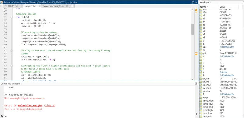
The function name and the output in the same function differed.

2. An error where the code was run with temperature values from the global range, which was later commented and a new 'T' was created with local temperature range.

3. Errors with missing and mismatching brackets, typos were also encountered.

Results/plots-

1. O2 -

2. N2 -

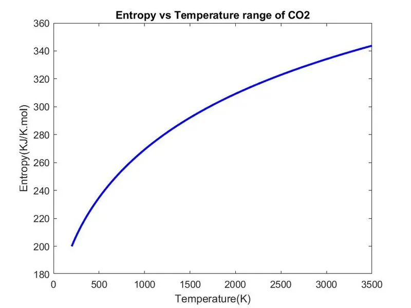
3. CO2 -

Molecular weights of all the species -