Week 1- Mixing Tee
Aim - To simulate and compare the mixing effectiveness of two free streams at different temperatures and velocities in a T-section pipe on CFD Fluent with the help of k-ε model and SST k-ω model.
Introduction - A T-section pipe is a component used commonly in systems where fluid flow takes place. Few of the systems for example are air conditioning unit, refrigerators, etc. In this project in particular we are putting into use two differently dimensioned T-sections to compare the efficiency of mixing and incorporate two CFD turbulence models and check their efficiency with the given problem. The turbulence models are the k-ε model and the SST k-ω model(SST stands for Shear Stress Transport). Here we have two cases one being the T-section with shorter pipe than the other. Each case will be simulated with two momentum ratios(momentum ratio = velocity at cold inlet/velocity at hot inlet). The fundamental job is to create a steady-state simulation to compare the mixing effectiveness when hot inlet temperature is 360C and the cold inlet temperature is at 190C.
Theory -
In order to compare the results from the two turbulence model lets discuss them individually to have a broad understanding of how both the models differ and how significant they are for a particular problem.
The k-ε model - The k-ε model is one of the most common turbulence models, albeit it doesn't perform quite well in cases of large adverse pressure gradients. The name k-ε is coined because it is a two equation model which includes two extra transport variables viz. 'k' and 'ε'. The variable 'k' represents turbulent kinetic energy which determines the energy in the turbulence whereas the second variable 'ε' represents the turbulent dissipation which determines the scale of the turbulence. The k-ε model has been shown to be useful for free-shear layer flows with relatively small pressure gradients. Similarly, for wall-bounded and internal flows, the model gives good results only in cases where mean pressure gradients are small; accuracy has been shown experimentally to be reduced for flows containing large adverse pressure gradients.
The SST k-ω model - The k-ω model is one of the most common turbulence models, this model similarly is also a two equation model with two extra transport variables viz. 'k' and 'ω'. Variable 'k' represents the turbulent kinetic energy determining the energy in the turbulence whereas 'ω' represents the specific dissipaton of turbulence which determines the scale of the turbulence.
Coming to the term SST which stands for 'Shear Stress Transport' is a model that combines our two basic models i.e. the k-ε and the k-ω model such that the k-ω is used in the inner region of the boundary layer and switches to the k-ε in the free shear flow.
Why do we need an SST model?
In simple language the SST model combines the best of both worlds while solving. The use of a k-ω formulation in the inner parts of the boundary layer makes the model directly usable all the way down to the wall through the viscous sub-layer. SST stands for shear stress transport. The SST formulation switches to a k-ε behavior in the free-stream, which avoids the k-ω problem of being sensitive to the inlet free-stream turbulence properties. This model serves best for adverse pressure gradients within the flow.
Solving and Modelling approach -
For Case - 1 with short mixing T-section we will simulate it with k-ε model and k-ω model SST.
For Case - 2 with long mixing T-section we will use the appropriate model based on our observations from previous case results.
Each case will be simulated with two values of momentum ratios.
The CAD model for the component is developed using Spaceclaim.
Mesh creation is done on Mesh Workbench.
CFD fluent on Ansys Workbench will be used for solving the equations and generate appropriate graphs.
Post-processing will help us generate contours and charts for temperature and velocity across various planes of the component.
For us to know whether the k-ε or the k-ω model is better we will try solve and simulate the first case with momentum ratio = 2 in both the models and find out what data is better to save time and achieve accuracy simultaneously.
To measure accuracy of the mixture temperature we have a theoretical formula to compare with, it is given as,
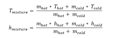
The first case includes a short T-section with momentum ratio = 2
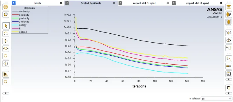
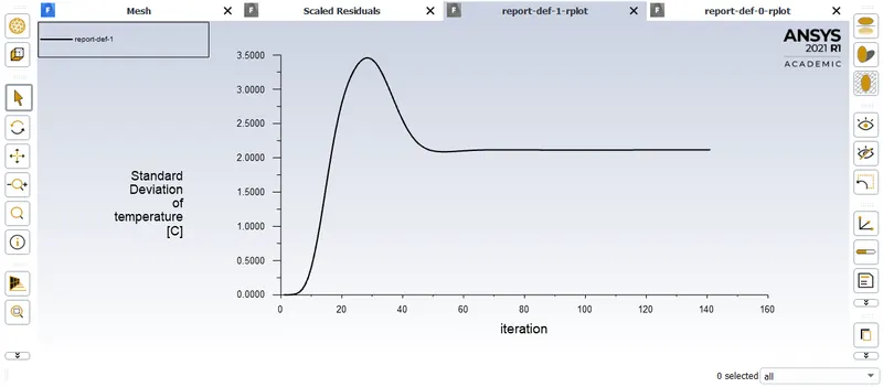
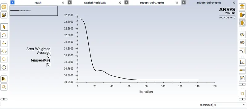
We will generate a residuals plot, an area weighted average of temperature at the outlet and a standard deviation of temperature at the outlet using k-ε and then the k-ω model leading us to a comparison for selection of a better model for further cases. Element size while meshing in both models were equal to 1.5mm. Below this value the element count crosses the academic license restriction, hence careful meshing has been performed in all the further cases to keep element count below 512000.
Data extracted using k-ε (realizable) model -
Residuals plot-
Standard deviation plot-
Area weighted average plot-
Out of 200 iterations the solution was converged at iteration 141
The computational time was not significantly less however it saved some.
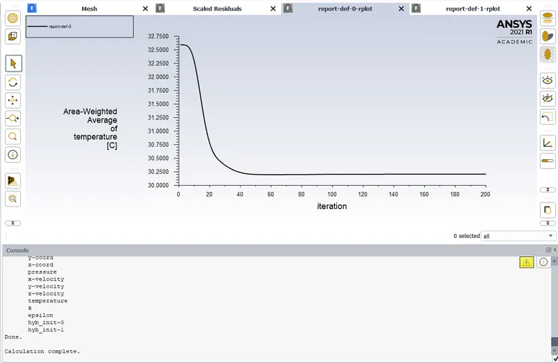
Average temperature at the outlet is 30.30°C.
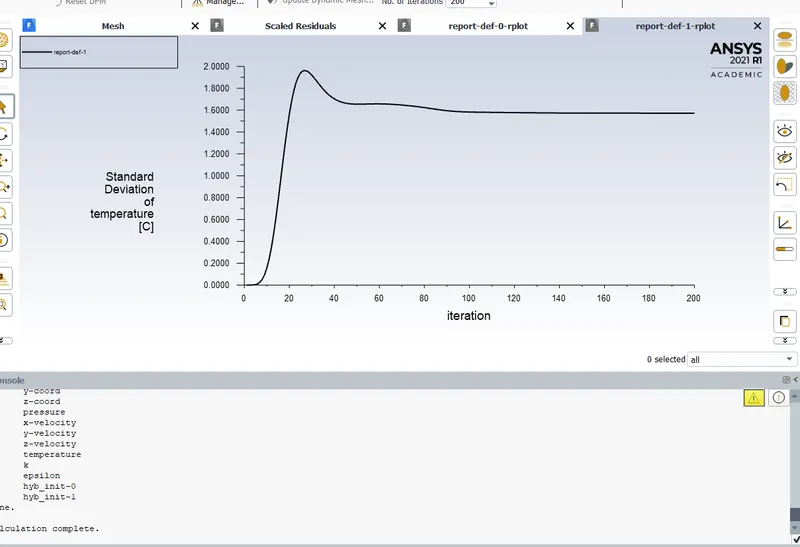
Standard deviation of temperature at outlet is 1.5
Data extracted using k-ω (SST) model -
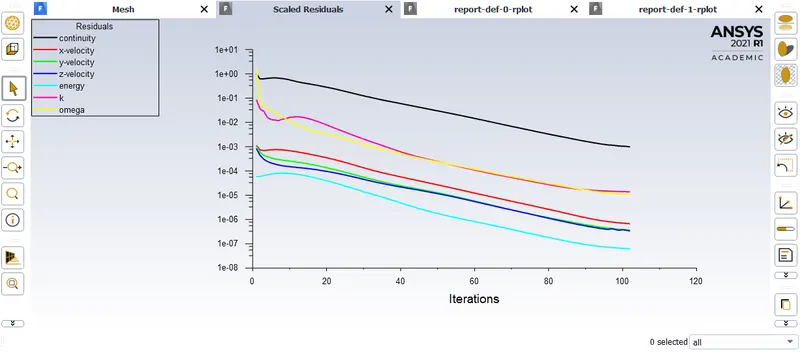
Residuals plot -
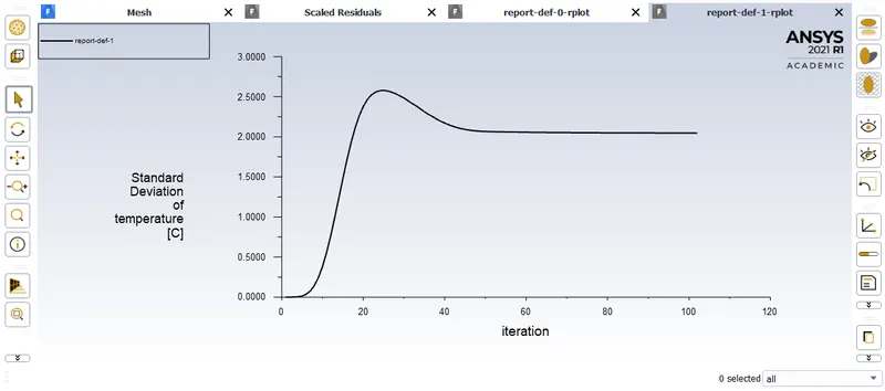
Standard deviation plot -
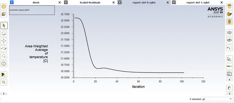
Area weighted average plot -
Out of 200 iterations the solution was converged at iteration 102, hence saving a significant amount of computational time.
Average temperature at the outlet is 30.45°C.
Standard deviation of temperature is 2 which is a bit on the higher side in comparison to the k-ε model.
However, the k-ω model saves a lot of time and the average temperature obtained is also closer to the theoretical value by decimals i.e. 30.77°C(a snippet of which has been attached in the later part of this report).
For a better accuracy and lesser time consumption opting for k-ω (SST) model will be wise.
Hence, all the cases further solved and simulated will be incorporated to the k-ω model.
Pre-processing and solver setting -
Geometry of the component has been loaded on Spaceclaim.
The geometry is of simple nature, has two inlets, one cold and the other hot, with a single outlet.
The cold inlet is closer to the hot inlet where both the air(hot and cold) enters and mixes well inside the cylindrical wall/pipe before passing through the outlet.
All of the three openings have an extension to their circumferences for assembling purpose which has to be neglected while meshing and further solving otherwise can increase our element count for no good reason and also increase the computational time to some extent. This construction at the openings is not deleted from the original geometry but the rest of the construction that is an important part of the meshing phase is extracted and the rest is suppressed while inserting in the solver by selecting the 'suppress for physics' option. 'Volume extraction' is used for extracting the necessary construction.
Geometry in Spaceclaim for Case-I before volume extraction-
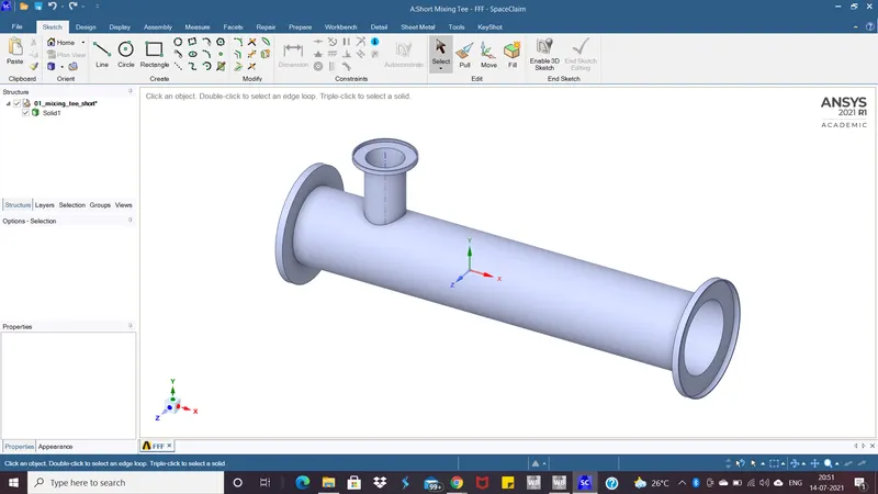
After necessary volume extraction-
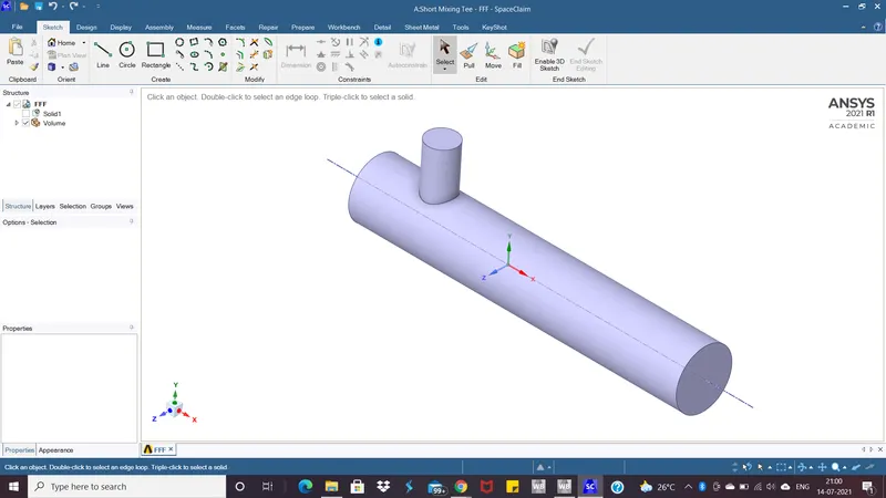
Spaceclaim is exited while the component changes are automatically saved and ready for Ansys Mesh as an input.
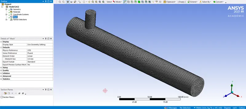
Ansys Mesh is started up and the geometry gets loaded, as a part of comparison study the meshing is initially done with the default element size and then refined accordingly.
In addition to this procedure the element number has to be kept under 512000 due to license restriction.
After the component is completed loading the 'Face select' option is activated and each face is named as per their existence, viz. inlets, outlet, walls. These names will be very helpful in the Fluent interface since Ansys identifies these names and assign them functions accordingly while solving the continuity equations.
Component in Ansys Mesh -
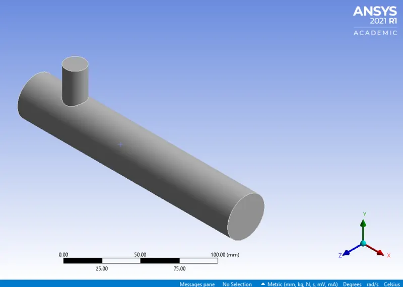
The mesh is generated with the default element size -
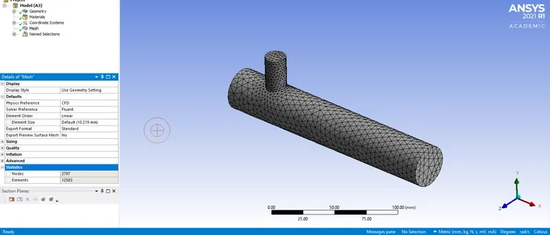
Evidently the meshing is not quite refined but for a better understanding of how a solution is affected by element size we will use this particular mesh and proceed with forming the solutions, contours, graphs and other data.
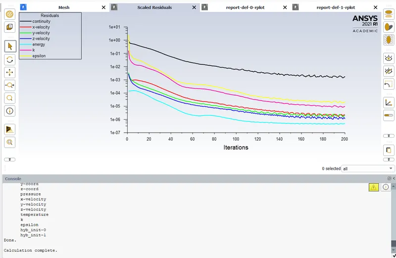
The Residuals plot-
The Area weighted average of temeprature at outlet plot-
The standard deviation of temperature plot -
The results in the form of X-Y graph would not be that intuitive as we can see, therefore we will move forward with setting up temperature and velocity contours in the post processing interface to have a look of the data distribution.
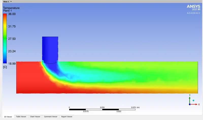
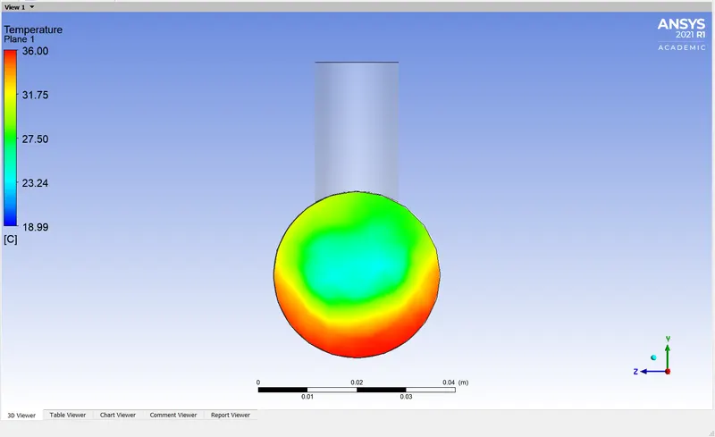
The temperature contours in the XY and YZ plane respectively-
The velocity contours in the XY and YZ plane respectively-
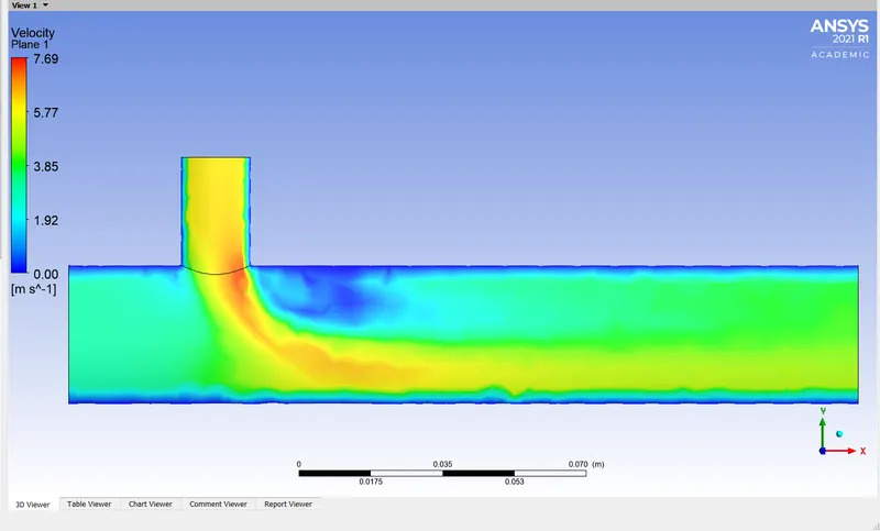
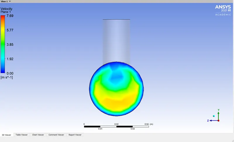
By the look of it we can say that the colour distribution in the contours is somewhat spready and is not refined due to lesser number of elements generated in the meshing phase. After identifying that the meshing has to be refined to capture more details of temperature and velocity disitribution, we can exit the post-processing phase or the 'Result' and boot the Ansys Mesh to edit the element size.
Now we can carry out with the Cases for the T-section with refined element sizes.
Different element sizes are used in every case for comparing results and contours and understand the mesh dependency of a model. A complete Mesh independent study has also been carried out later in the report.
Case-I a - Short T-section with momentum ratio = 2
Geometry of the Short T-section has been showed with the help of snippets above. The necessary volume extraction is carried out for ease in meshing and solving, additonally saving us computational time. Spaceclaim is exited while the construction saves itself automatically and loads in Ansys Mesh.
After meshing with the default element size we observed that the simulation was missing intricate details in the colour distribution for velocity and temperature contours. For this case we will set the element size to 1.5mm and generate the mesh, for which the result looked like in the below image.
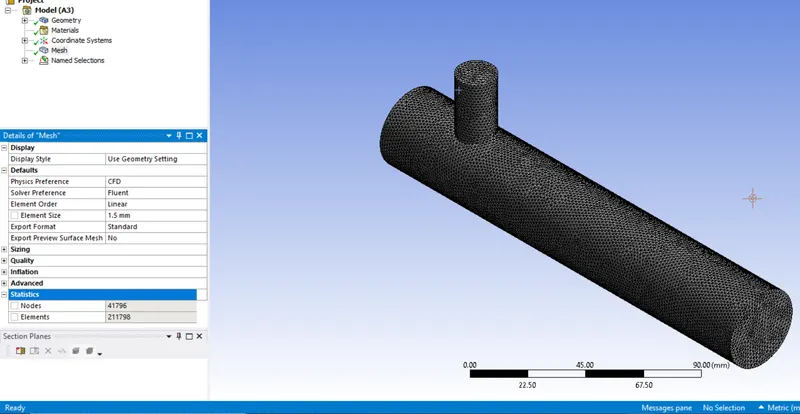
The meshing here looks quite refined and would suffice for the details needed from the contours.
Now the Fluent(Setup) is accessed for necessary plots.
Before commencing the solving of equations the solver requirements are fulfilled, it includes-
1. Setting up the units to our preferences.
2. Ticking for the energy equation to include temperatures and its input.
3. Selecting the appropriate model, k-ω SST in our case from the viscous model.
4. Giving the temperature and velocity inputs in the boundary conditons.
At the hot inlet that is the inlet along the x-axis the velocity of air entering is 3m/s and its temperature is 36°C.
While at the cold inlet that is the inlet normal to the x-axis the air entering is at 6m/s at the temperature of 19°C.
5. Setting up plots for area weighted average and standard deviation through surface reports.
Residuals plot -
As we have used the Short T with momentum ratio = 2 case for selecting a better model between k-omega and k-epsilon, this is the same plot with 102 iterations performed until its convergence out of the 200 entered.
Area weighted average of temperature at the outlet plot -
The average temperature at the outlet is 30.45°C.
The standard deviation of temperature at the outlet -
Standard deviation is equal to 2.
Results-
For the post-processing part the 'Results' is booted on the Workbench.
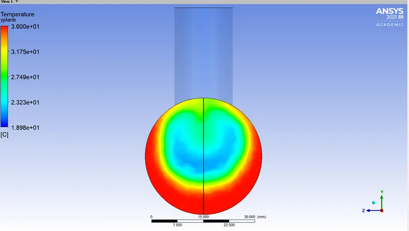
The cylindrical walls are displayed and the rest of the parts that are the inlets and the outlet are disabled. The walls are made transparent enough for us to have a clear visibility of the contour planes generated in it.
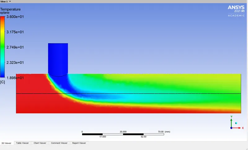
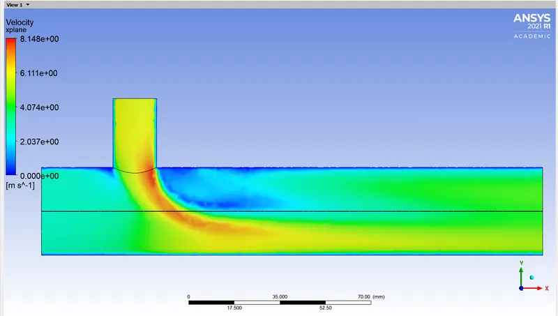
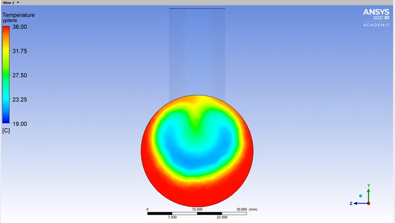
Two planes are generated in the component, one along the pipe (along the x-axis) and the other across the pipe (normal to the x-axis). Each of the planes will be coloured by a variable, temperature and then velocity.
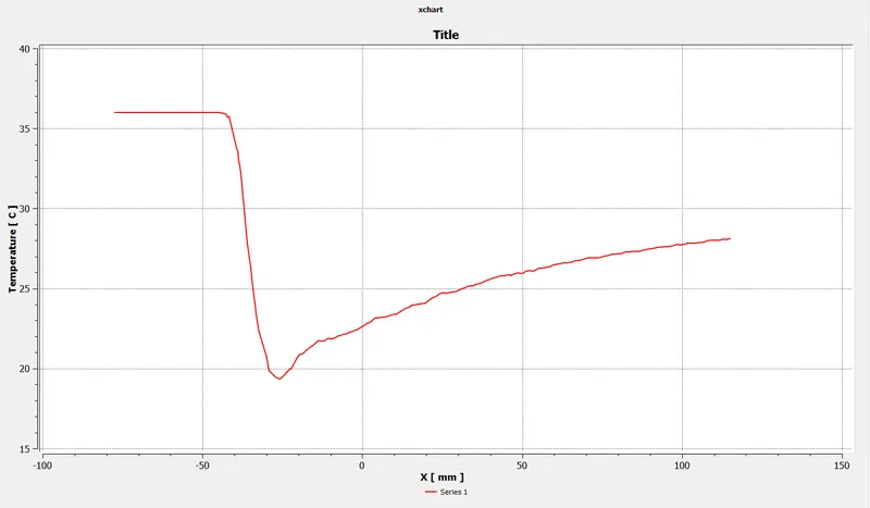
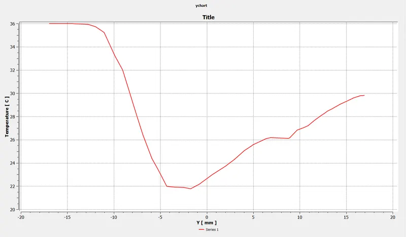
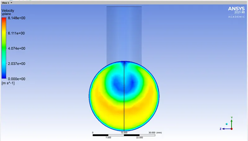
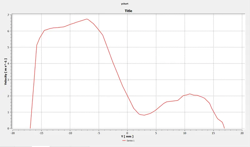
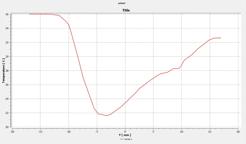
Now to get our hands on the specific data values from the contours in terms of numbers and units, a line passing through the plane in the same behaviour as the plane's with respect to the x-axis can serve the purpose.
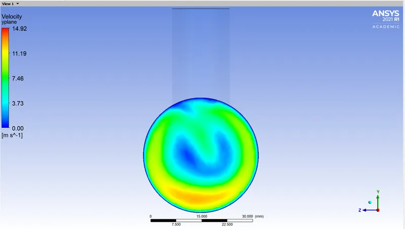
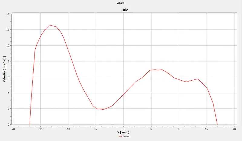
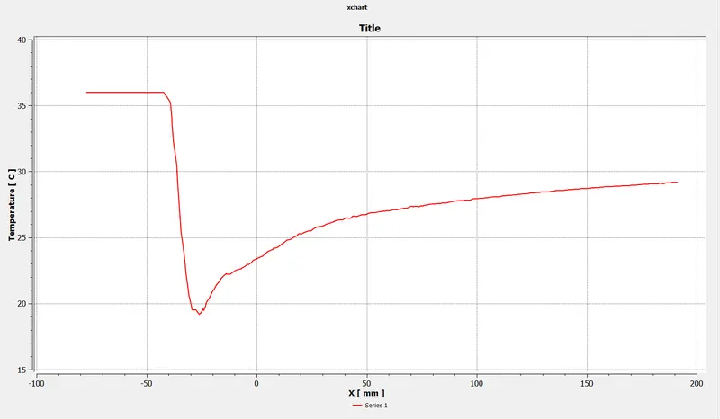
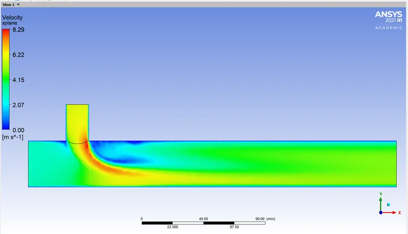
The values are then displayed in terms of charts as X-Y line graph for each parameter in both the directions.
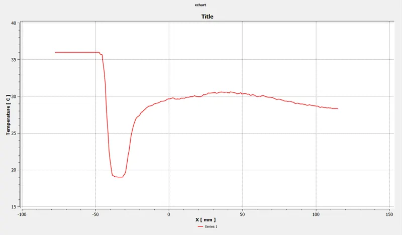
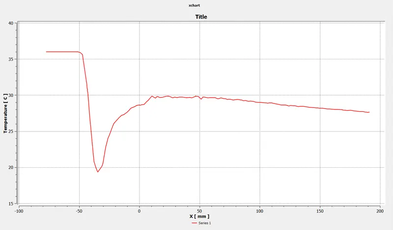
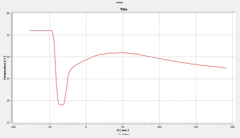
The temperature contour and graph along the pipe-
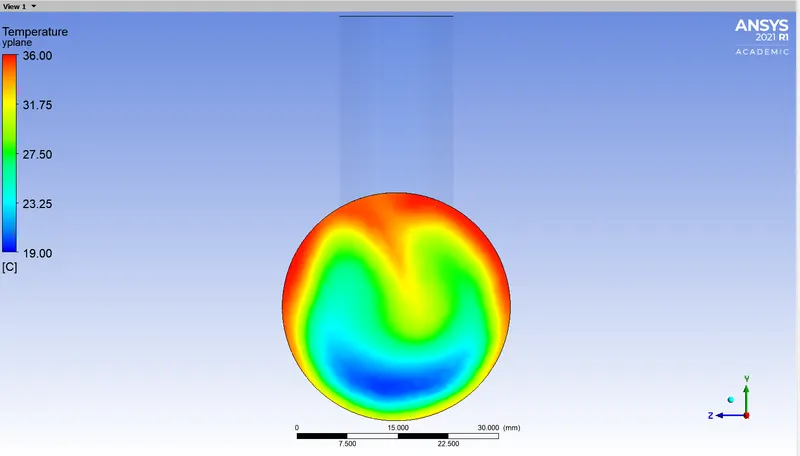
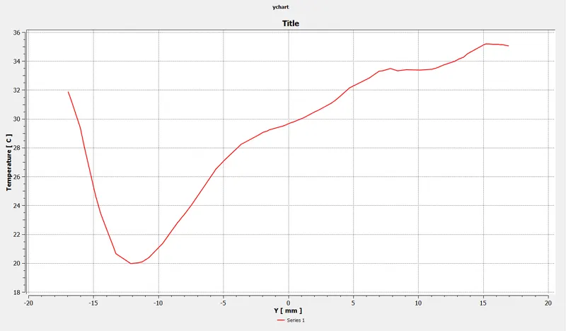
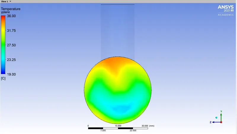
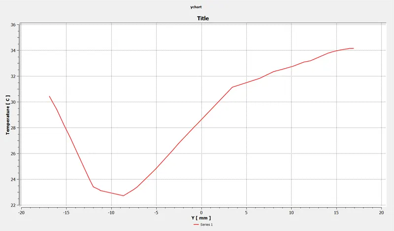
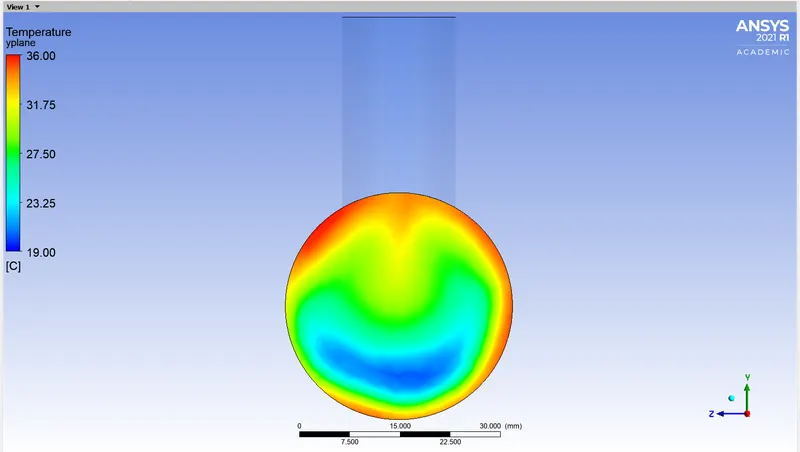
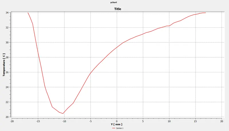
The temperature contour and graph across the pipe -
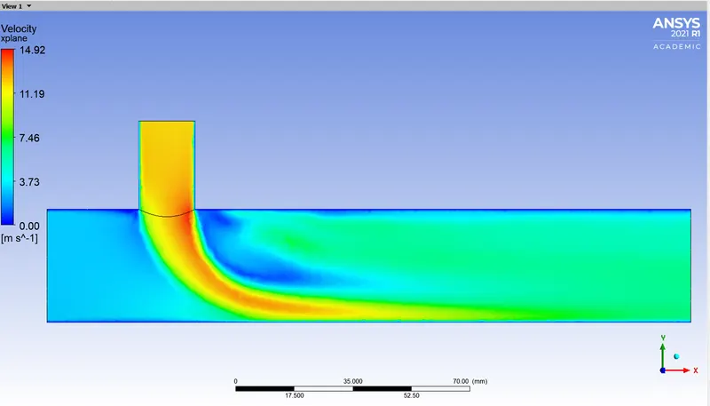
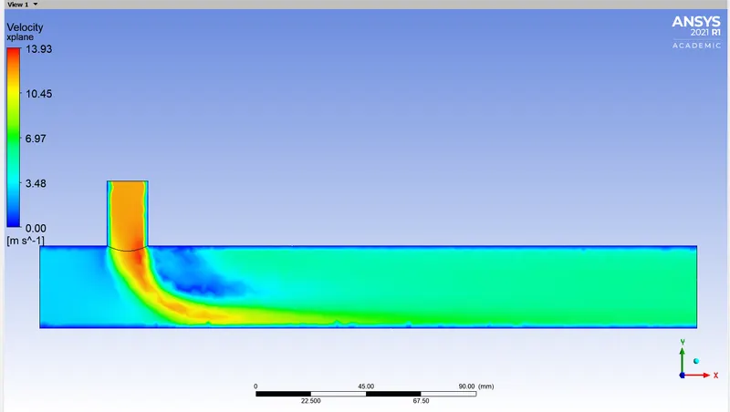
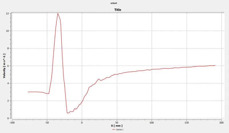
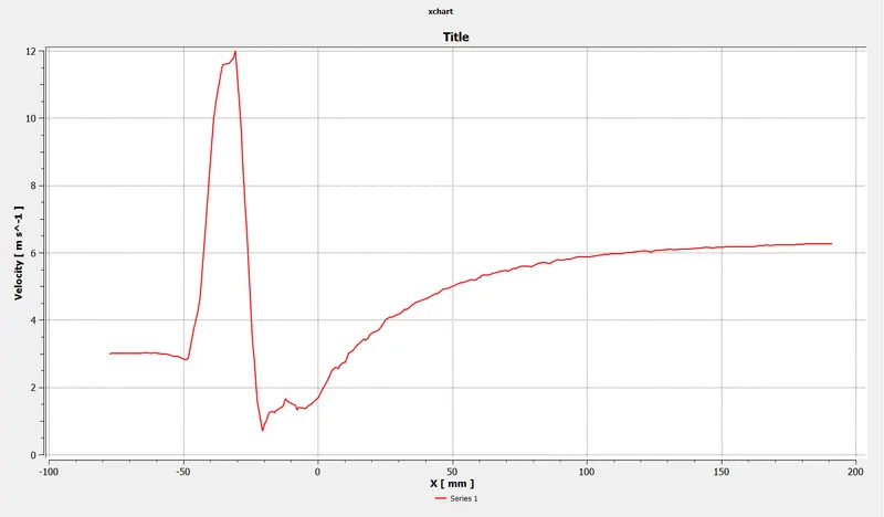
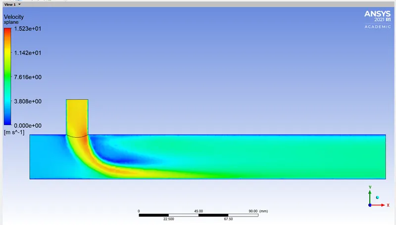
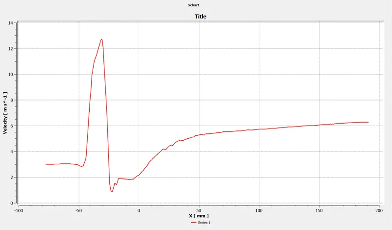
The velocity contour and graph along the pipe -
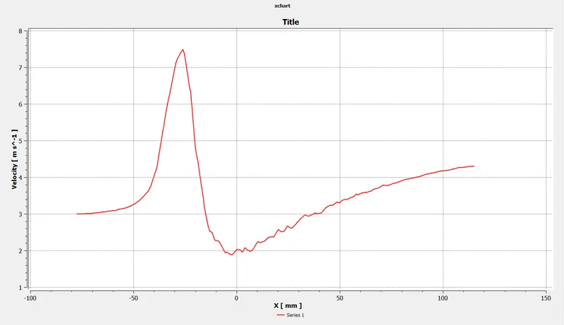
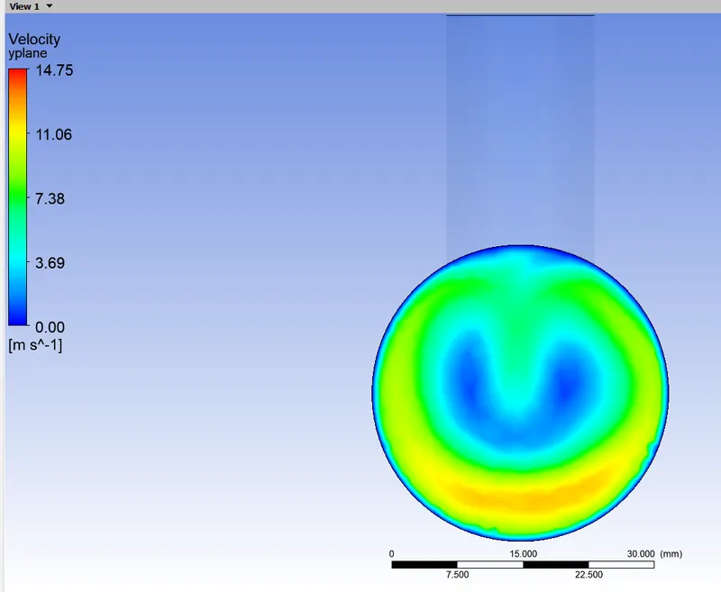
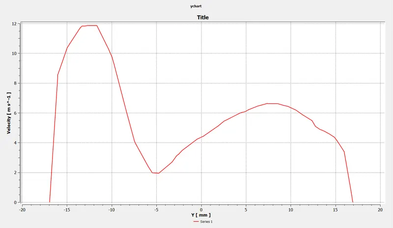
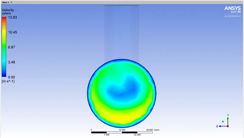
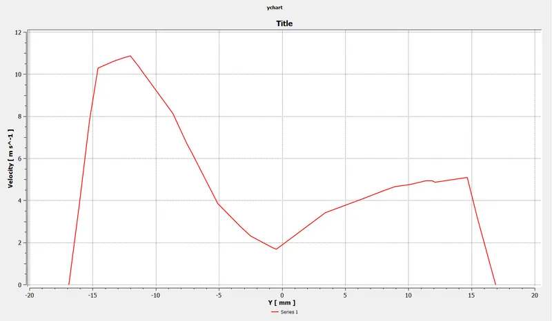
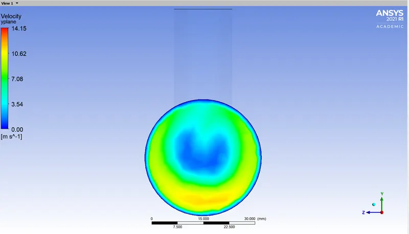
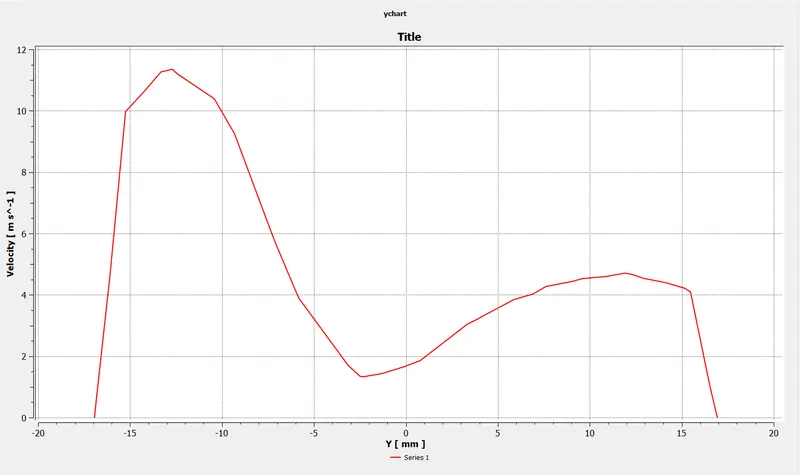
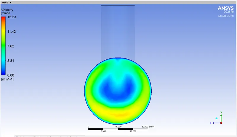
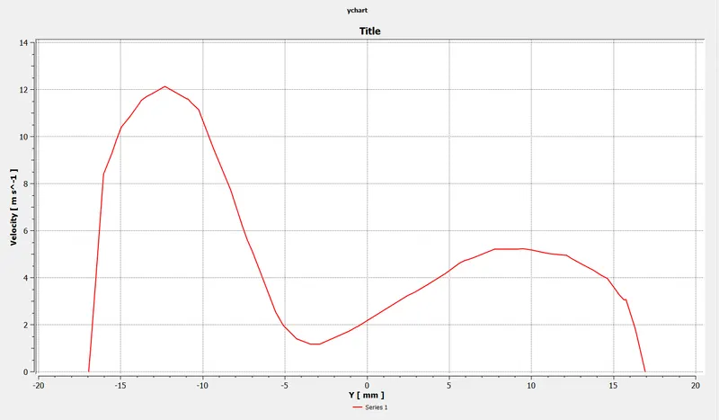
The velocity contour and graph across the pipe -
Case-I b- Short T section with momentum ratio = 4
Geometry of the component remains the same in Spaceclaim.
Whereas in Ansys Mesh the meshing is made even finer to 1.1mm, keeping an eye on the element count, under 512000.
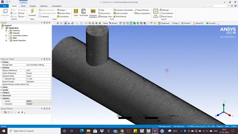
In the Ansys Setup the velocity at the cold inlet has been now changed to 12m/s and the rest of the inputs remains unchanged.
Three plots has been generated same as the previous case.
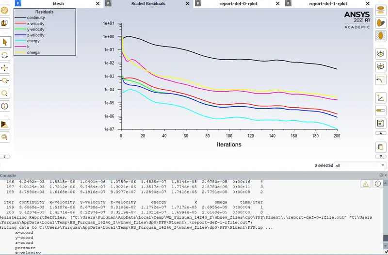
The residuals plot-
The standard deviation of temperature at outlet plot-
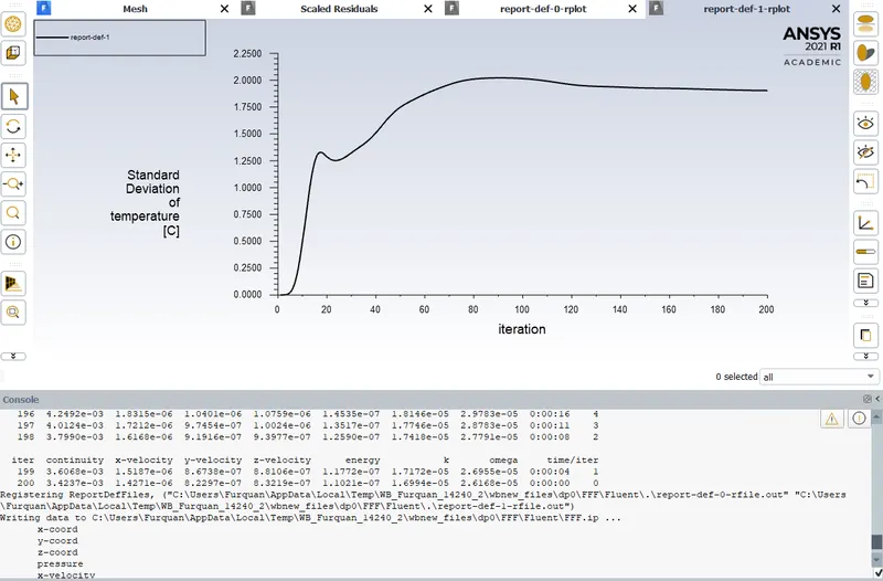
The standard deviation is 1.65.
The area weighted average of temperature at outlet-
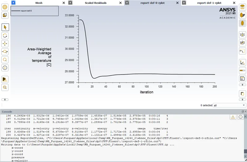
The average temperature at outlet is 27.5°C.
Moving on to the Post-processing phase the respective contours and graphs are generated.
The temperature contour and graph along the pipe-
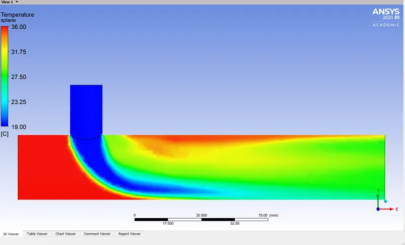
The temperature contour and graph across the pipe -
The velocity contour and graph along the pipe -
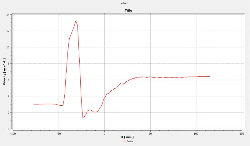
The velocity contour and graph across the pipe -
Case-II - Long T-section with momentum ratio = 2
The only change in the Geometry section is the length of the cylindrical wall, which has been increased. In other words the distance between the hot inlet and the outlet is increased.
The entire process of volume extraction is carried out in Spaceclaim and then loaded in Ansys Mesh.
Mesh is generated with element size=1.2mm
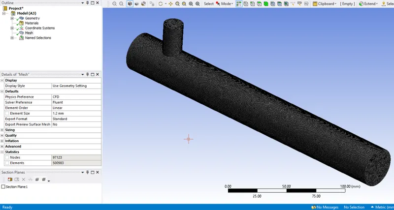
Since the component has its volume increased compared to the shorter one the element size was increased by 0.1mm i.e. 1.2mm to keep element count under threshold value(512000).
The faces are selected and named accordingly in the same way as the short T.
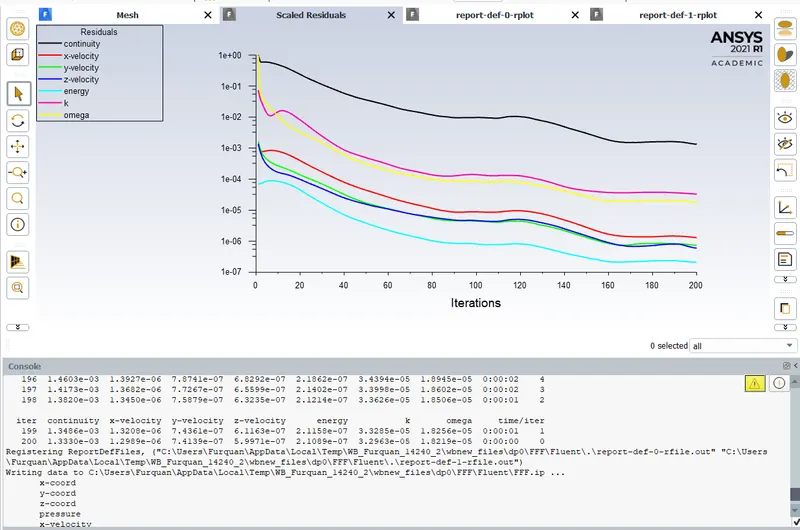
Ansys Fluent is booted and the component is loaded, every step is carried out same as the Short T-section with the cold inlet velocity as 6m/s, and the required plots are generated. All of the 200 iterations are performed from the 200 entered.
The residuals plot-
The standard deviation of temeprature at outlet plot-
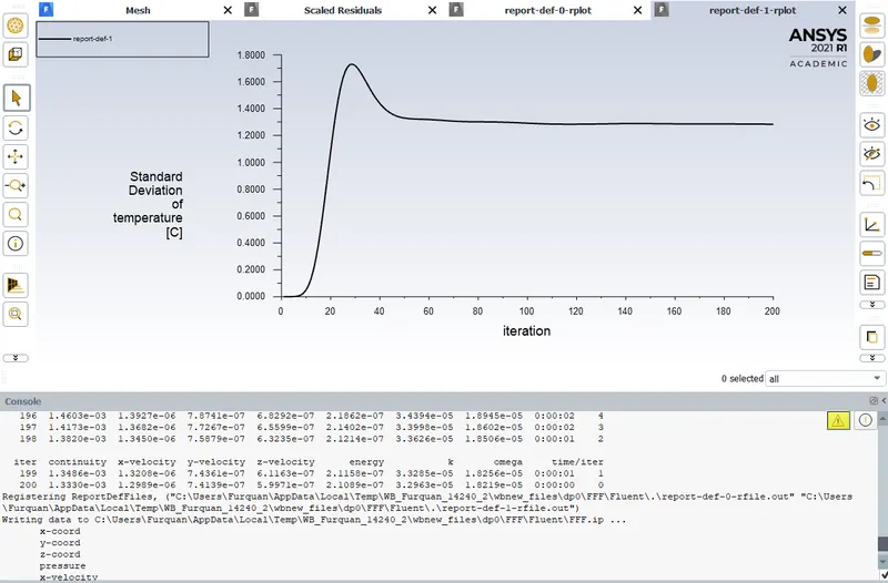
The standard deviation is 1.3, quite closer to being 1.
The area weighted average of temperature at outlet-
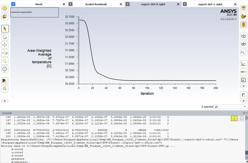
The average temperature at the outlet is 30.35°C.
After the Setup and Solution for the simulation is ready the Results section is booted for generating contours and graphs.
The temperature contour and graph along the pipe-
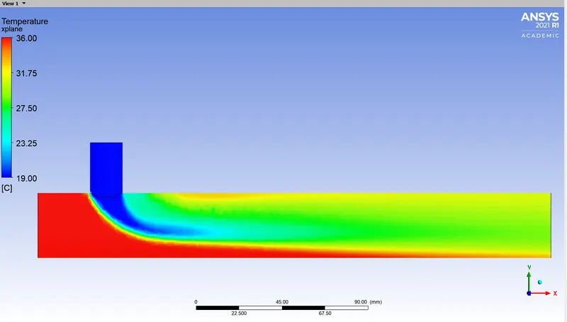
The temperature contour and graph across the pipe -
The velocity contour and graph along the pipe -
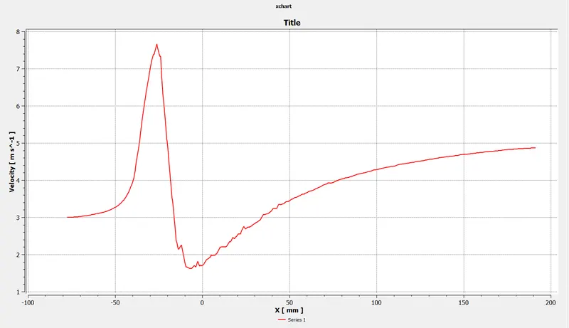
The velocity contour and graph across the pipe -
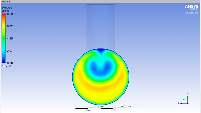
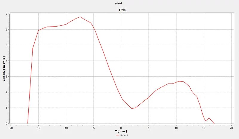
Case-II - Long T-section with momentum ratio = 4
Now the cold inlet velocity has been changed to 12m/s in the boundary conditions and the rest of the procedure was kept unchanged.
The residuals plot-
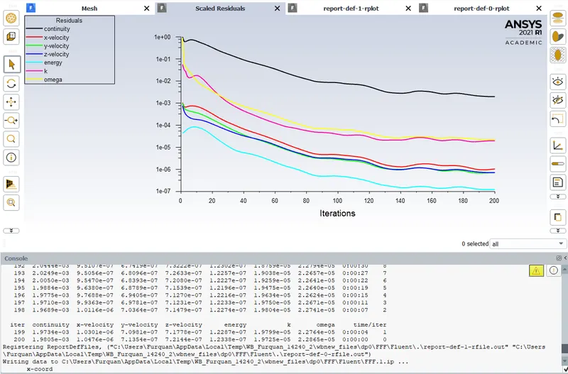
The standard deviation of temperature at the outlet plot-
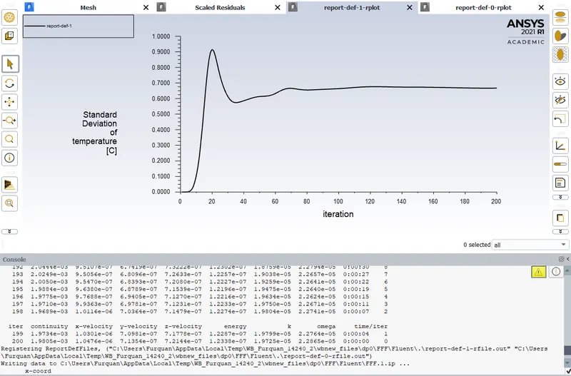
The value for standard deviation is 0.65, which is the closest we have achieved towards zero.
The area weighted average of temperature at the outlet plot-
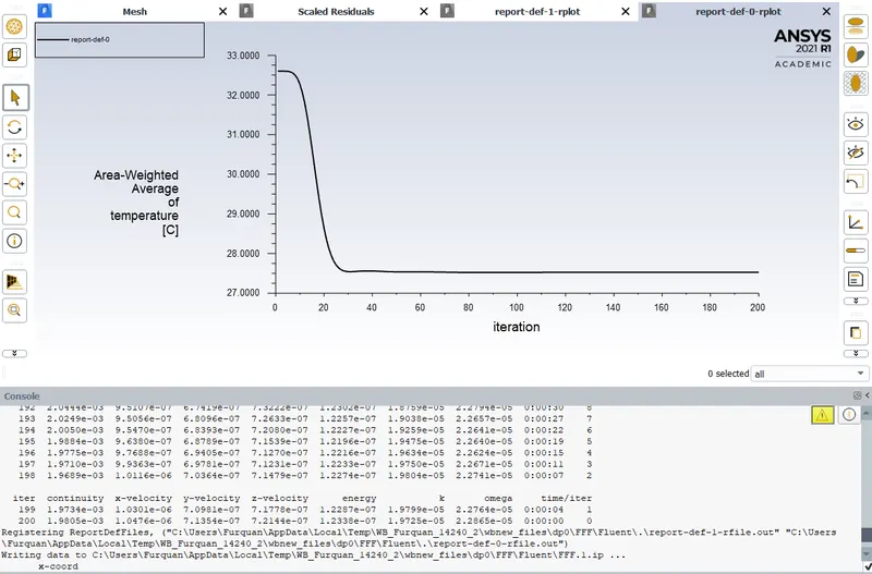
The average temperature at the outlet is 27.5°C.
The velocity and temperature contours generated-
The temperature contour and graph along the pipe-
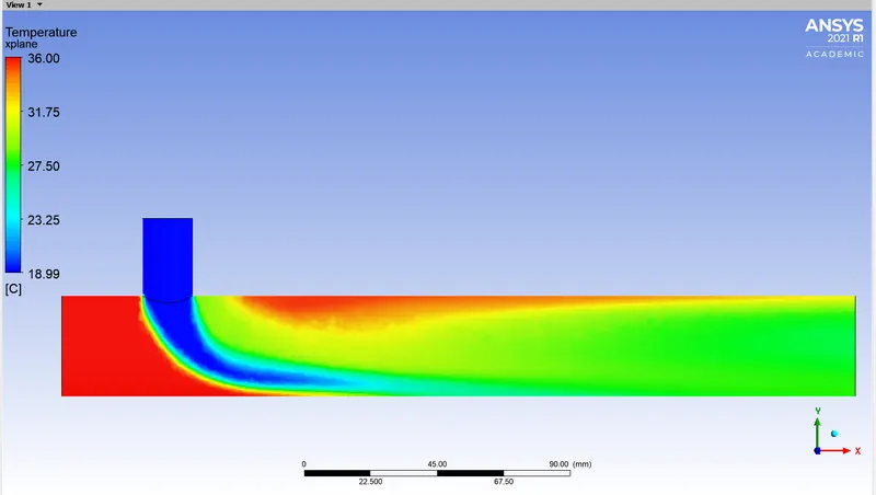
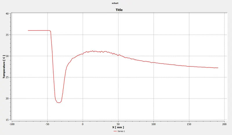
The temperature contour and graph across the pipe -
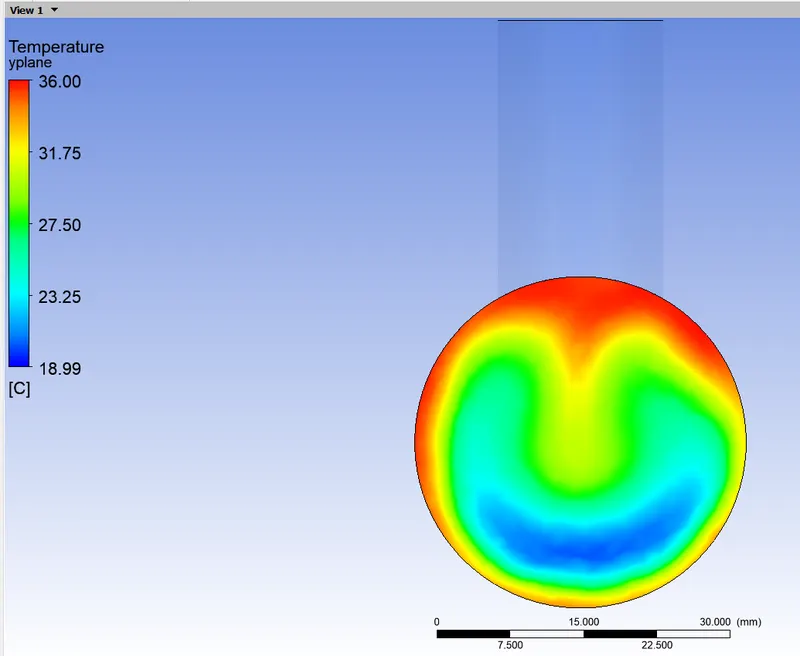
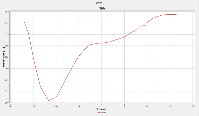
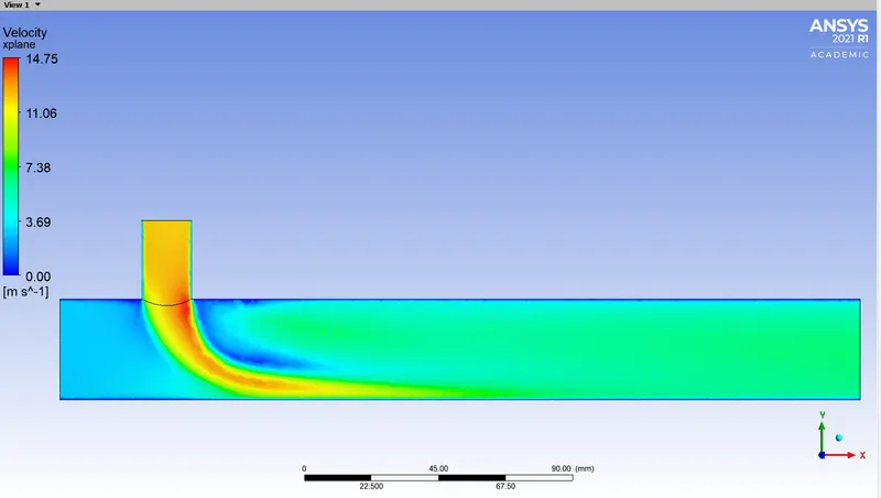
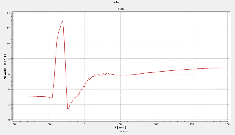
The velocity contour and graph along the pipe -
The velocity contour and graph across the pipe -
Conclusion-
Firstly, lets discuss about the effect of momentum ratio for each T-sections.
Temperature contour for short T with MR=2(left) and MR=4(right).
When we observe the temperature contours for the Short T with different momentum ratios we can say the mixing is efficiently taking place in the case with the higher momentum ratio. It is evident for the contour with MR=2 at the outlet that the hot air entering from the larger inlet does not entirely mixes with the cold air and leaves the outlet as it were while entering. This issue can probably be solved by giving the hot air a little more time to mix with the cold air, since the boundary of the gradually passing hot air seems to be decreasing proving us that it would eventually mix up if the pipe length were to be longer. Lets have a look at the temperature contour for long tee with MR=2 to try proving this theory.
Temperature contour for long tee with MR=2
We can say that the theory is really close to be correct, since this seems to be a better result with a better mixing efficiency at the outlet with MR=2 in comparison to the short tee with the same momentum ratio. However the result with an MR=4 in a short T is more satisfying i.e. to increase the celocity of cold air entering.
To accomplish our goal that is to obtain a good mix of both the air is by making it flow through a long T at a momentum ratio of 4, lets compare a long tee temperature contour with momentum ratio of 2 and 4.
Temperature contour for long tee with MR=2(left) and MR=4(right).
By looking at the outlet of the contour with MR=4 the temperature is quite stable for some length and the mixing is done well.
If we consider our long T at MR=4 as our ideal model lets compare the value at the outlet which is 27.5°C from the area weighted average plot with our validation value obtained from the formula given in the initial part of this report discussed in the 'Solving and Modelling approach'.
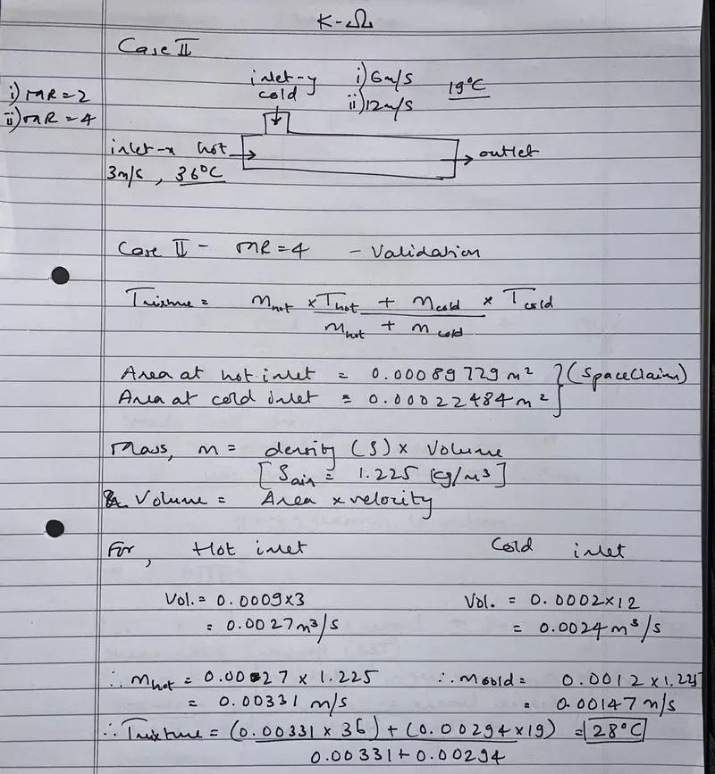
The validation value obtained is 27.5°C which is very close to the simulation value.
Similarly we can compare the simulation and validation values for temperature for all previous cases, here is a table for the same,
Table 1-
| Momentum Ratio | Simulation value (°C) | Validation value(°C) | |
| Case-I | 2 | 30.45 | 30.77 |
| 4 | 27.5 | 28 | |
| Case-II | 2 | 30.38 | 30.77 |
| 4 | 27.5 | 28 |
It will be safe to say that in every case the velocity is uniform along the cross-section at the outlet.
To justify our first case with MR=2 with 102 iterations being performed out of the 200 entered are the number of cells which is significantly lesser than the other cases, less than half to be fair. This is due to the solver which is solving the continuity equations for every cell quicker due to lesser elements and lesser time required for them to be solved and sooner it will have a consistent solution due to which the solver quits solving the equations and claims the model to be converged.
As we observed that longer the pipe better the mixture at the outlet, on the contrary increases the element count and consequently the computational time. However on the brighter side we will achieve a better mixture with an intricate model simulated at our display.
A table for comparing various data obtained among the cases is generated,
Table 2-
| Momentum Ratio | Cell count | Average outlet temperature(°C) | Number of iterations for convergence | |
| Case-I | 2 | 211798 | 30.45 | 102 |
| 4 | 456020 | 27.5 | 200 | |
| Case-II | 2 | 500983 | 30.35 | 200 |
| 4 | 500983 | 27.5 | 200 |
Mesh independent study -
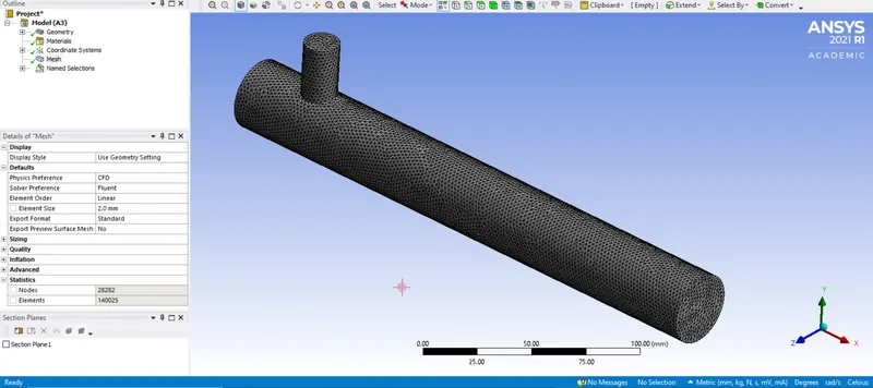
The mesh independent study has been performed on the Long T with MR=4 using a k-ε model. All the data shared via graphs and charts are in the same fashion as the cases taken previously for mixture study.
Case-I for element size = 3mm
Case-II for element size = 2mm
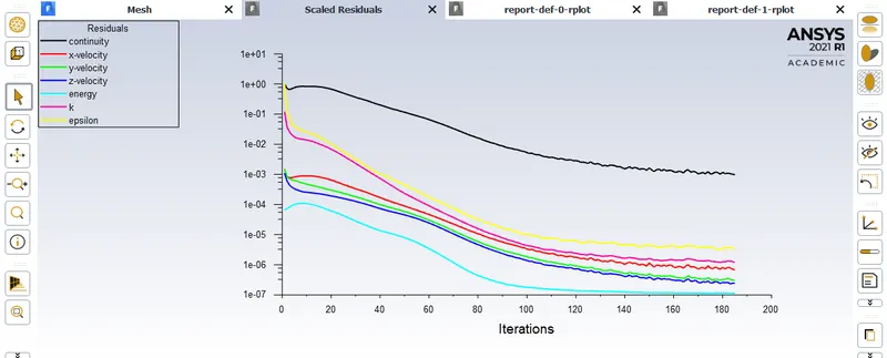
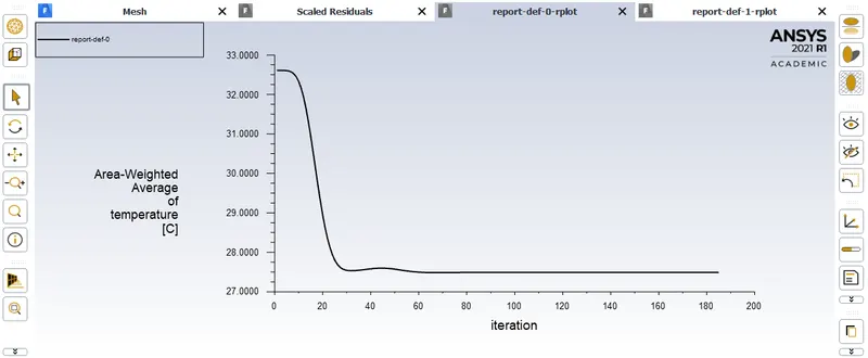
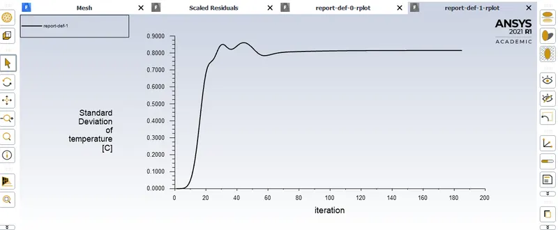
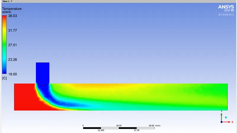
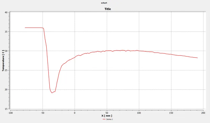
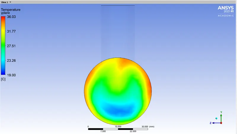
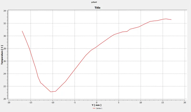
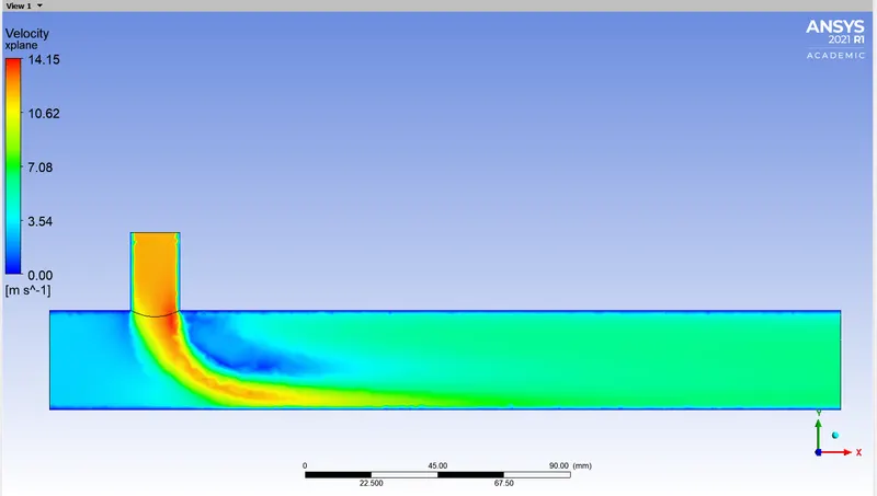
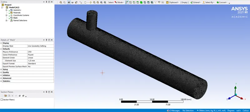
Case-III for element size = 1.25mm
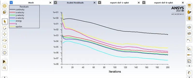
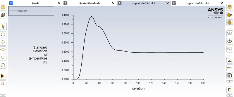
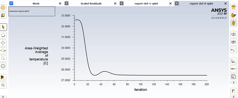
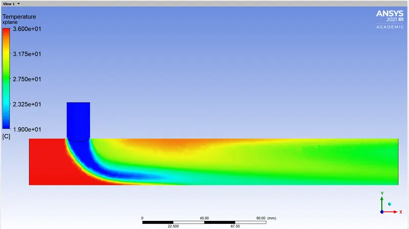
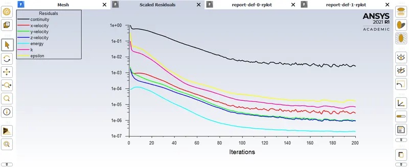
The scaled residuals in all the cases are mostly behaving in a similar manner.
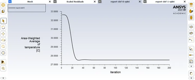
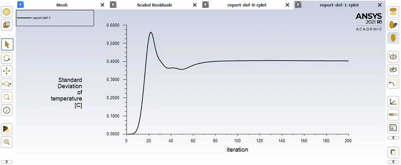
Although the standard deviation is different in each case, the average temperature is quite the same in all the three plots, which indicates that the model is mesh independent.
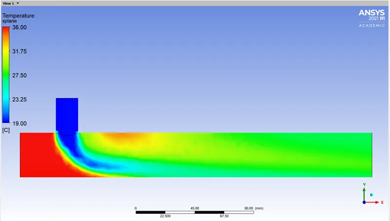
The contour has the exact same colour distribution with the only difference in details, where for every decrement in element size the contour gets refined alongwith the mesh.
To conclude, the T-section is one of the most commonly used component in engineering and industrial engineering. Simulation of this section with different values and tweaking it for every digit can give us better solution or on the opposite side worse. This approach can help us thrive towards an optimal solution before applying it in the bigger system for practical application.