Week 2 - Flow over a Cylinder.

Aim-

PART-I

To simulate a flow over cylinder and calculate Strouhal number for Reynolds number = 100 using a steady and transient solver sequentially.

PART-II

To calculate the co-efficient of drag and lift over a cylinder by setting the Reynolds number to 10, 100, 1000, 10000, 100000 with just the steady solver, discussing effects of Reynolds number on the co-efficient of drag by referring with a standard literature.

Introduction- A cylindrical object placed in an airflow produces a significant effect in the flow. This effect is well articulated and has been a topic of interest in the analysis domain. When this cylinder which will be demonstrated using Ansys will be kept or as to say created in such a way that generates a similar behaviour as a cylinder obstructing an airflow using Spaceclaim will cause a formation of multiple vortices adjacent to each other moving in the direction of the air flow. The source of these vortices is the part or face of the cylinder which is not exposed to direct contact of the airflow or rather the backside of the cylinder. The entire phenomena is called as vortex shedding. Vortex shedding occurs at a particular specification of the fluid i.e. the Reynolds number which then branches out to density, velocity, characteristic length and dynamic viscosity with respect to the general formula. Including Reynolds number there is another dimensionless parameter called as the Strouhal number which is by formula the product of frequency and characteristic length divided by the velocity of the fluid. Since we have all the values for our parameters but the frequency of the vortex shedding to determine the Strouhal number, we shall generate a lift co-efficient plot to calculate it.

Theory-

Vortex shedding-

Vortex shedding as a phenomena is simple physics that even occurs in our basic engineering applications. To simply understand imagine a block moving through fluid at a considerable velocity with two of the faces parallel to the flow and the other two normal to it. The block while moving will have the fluid hit in the front directly, now the rear side of the object has not yet been in contact with the fluid coming from the front. The fluid hitting on the front side creates higher pressure on the face than the face on the opposite side at the rear with lower pressure. Since the block is moving with a decent velocity the fluid tends to travel from the high pressure side towards the low pressure side due to vacuum at the back. When the fluid tries to fill the void or vacuum at the rear side it does so in a manner that looks like a vortex. An illustration shown below can explain better.

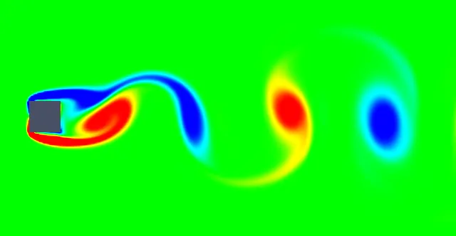
Vortex shedding for a cylinder-

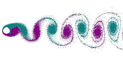
This repeating pattern of swirling vortices caused by vortex shedding gives a visual of multiple vortices aligned and moving is called as the Karman vortex street, named after an engineer and fluid dynamicist Theodore von Karman. It is a function of Reynolds number, and occurs typically above Re=40.

Strouhal number-

Strouhal number is a dimensionless number describing pattern in oscillating flow mechanisms, mathematically given as,

where,

St = Strouhal number

f = frequency of vortex shedding

L = characteristic length (diameter of the cylinder in our case)

U = velocity of flow

Drag and Lift-

A body moving through a fluid at a high velocity experiences two types of forces, one in the vertically upwards direction called lift and the other horizontally backwards called drag. The resultant of both the forces is considered to calculate the total aerodynamic force acting on the body. The term aerodynamic is used in case where roadway vehicles are analysed, whereas in the case of waterway transport such as a ship, boat or a submarine the term used is hydrodynamic force.

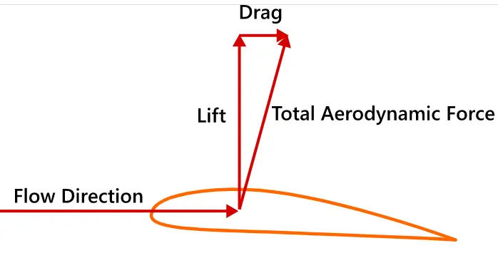
With this report the effect of Reynolds number on the co-efficients of drag and lift is determined. A cylinder placed in a fluid flow is the setup on which the various plots and contours are established.

Solving and Modelling approach-

A laminar model will be used for both the approaches to help simulate vortex shedding. The Reynolds number will be tweaked with the help of different velocity values. As the velocity is increased the Reynolds number increases. Other parameters such as the density, dynamic viscosity, characteristic length is kept constant, the values of which are,

density, ρ = 1 kg/mᶟ

dynamic viscosity, μ = 0.02 N.s/m²

characteristic length (dimeter of cylinder) = 2 m

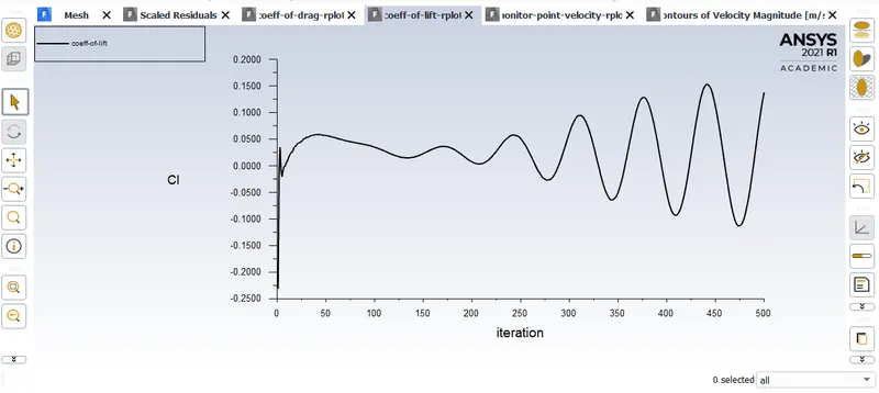
For Part-I, Strouhal number is calculated through a method, first by plotting a graph for the co-efficient of lift in a transient solver and then measuring the number of cycles in a given time period. Dividing the number of cycles wiht the its time span which will give the frequency of the vortex shedding. Since the only unknown has been calculated substituting this in the Strouhal number formula will give us its value.

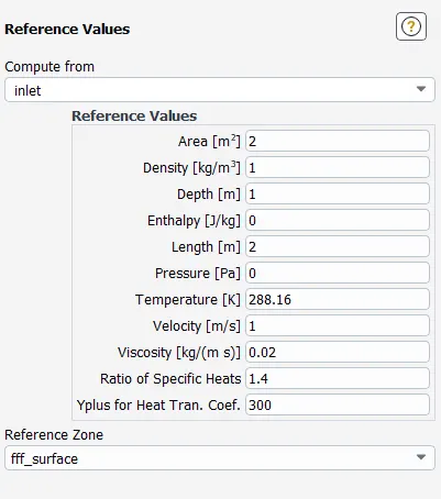
To get the correct values for drag and lift the reference values has to be changed to computing from the inlet and keeping the reference zone as the entire surface.

For Part-II, every Reynolds number value asked is achieved by changing the corresponding value.

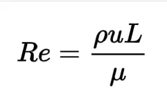
where, Re = Reynolds number

ρ = density of the fluid (kg/mᶟ)

u = velocity of the flow (m/s)

L = characteristic length (diameter for this cylinder) (m)

μ = dynamic viscosity of the fluid (N.s/m²)

Here all of the above parameters are fixed except for the velocity which will be changed for every Reynolds number value and also be the input in Ansys setup.

For example, if the need is a Reynolds number of 100 then,

100 = (1 x u x 2) / 0.02

∴ u = 1m/s

Pre-processing and solver setting-

Spaceclaim is used to achieve a similar situation to a top view of a cylinder placed in an environment.

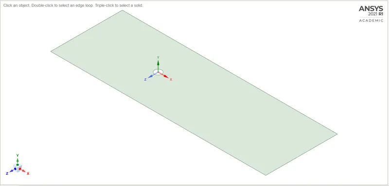
A simple circle is drawn over the XZ plane with diameter 2m and a rectangle around it of 60x20m with measured distances from the center of the circle to the rectangle edges.

The pull and select functions are used to keep the rectangle and remove the circle to make the geometry behave as a rectangular plate with a circular cut out, which is what is needed for the meshing and simulation.

After the geometry construction is ready it is loaded in Ansys Mesh. Initially after meshing the geometry with the default element size and generation the mesh loaded was coarse.

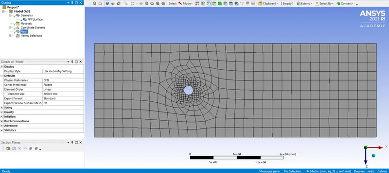
This mesh was refined with the help of certain functions, viz. inserting a method, the all triangle method which makes all the generated mesh predominantly triangle in shape; inserting the sizing, to improve the shape of the circle by giving more number of edges for it to look lesser like a polynomial; inserting inflation, a body shape meshing which basically means in this case concentric elements to the cylinder so that the details of the physical parameters is obtained around the obstacle placed on a fluid flow. Additionally the element size was set to 200mm and the result finally looked like,

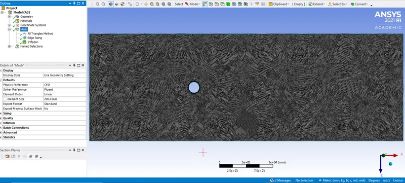
Named selection for the inlet, outlet, wall and symmtery is appropriately done.

Until this point the steps for both the parts remain the same. Now each part will be considered sequentially.

Ansys Fluent for Part-I (Re=100)

Case I - Steady solver

The Fluent setting includes the following

1. Using a steady state solver in the first case of this part
2. Setting the reference values appropriately as shown,
3. Keeping the Viscous Laminar model.
4. Creating a user defined material and defining its physics as per our requirement.
5. Setting up the boundary conditions where the velocity at the inlet is used as the input for our Reynolds number value.
6. Selecting the SIMPLE scheme method for steady state solver.
7. Generating the surface report of vertex average graph behind the cylinder using a monitor point at the same location.
8. Generating a force report of co-efficient of lift at the wall i.e. the cylinder to calculate the frequency of vortex shedding.
9. Using the standard initialisation option and setting to compute from the inlet.
10. After initialisation generate a velocity contour of the entire geometry and for the same contour an animation to have a better visualisation of how the vortex shedding occurs from the beginning to the end and hit calculate for 500 iterations initially and keep extending the process by calculating for another number of iterations until there is an evidence of Karman Vortex Street in the animation.

The Results-

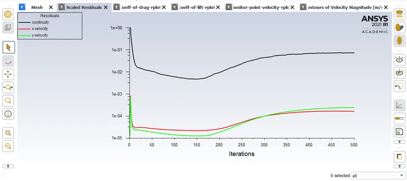
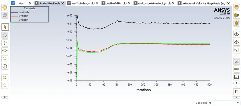
The residuals plot-

The vertex average of velocity plot-

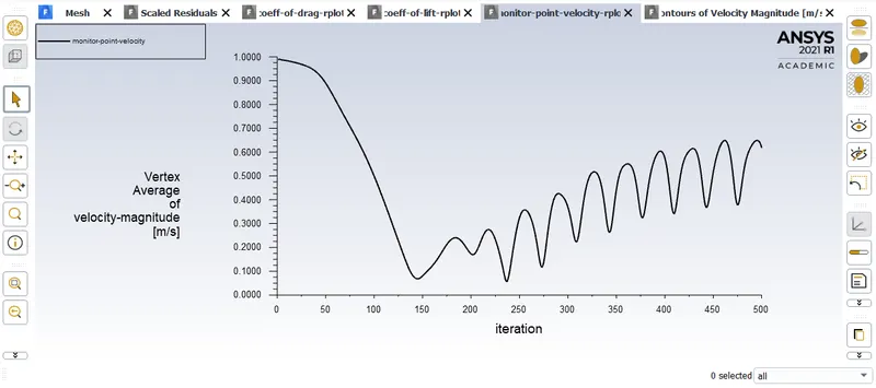
The start of fluctuations indicates that the vortex shedding has started.

The co-efficient of lift plot-

The velocity contour-

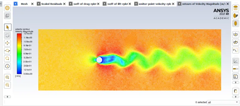
A perfect vortex shedding phenomena simulated in the above image.

An animation has also been produced attached to this report in the files section named 'anim-of-vel'.

Case II - Transient solver

Keep all the settings unchanged except for the solver, to the transient and the method to the coupled scheme method.

All the generated Results-

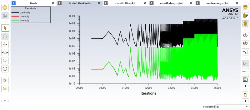
The residuals plot-

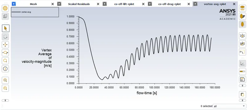
The vertex average of velocity-

The co-efficient of lift plot-

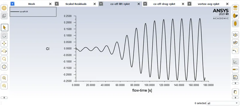
For calculating frequency the number of cycles in the time from 140 seconds mark to the 180 seconds mark is determined, which is 3 now the frequency is given by,

ω = 1.5 / (160 - 140)

= 1.5 / 20

= 0.075

∴ Strouhal number, Sr = (0.075 x 2) / 1

= 0.15

Hence, the Strouhal number is 0.15 for Reynolds number = 100 in a flow over a cylinder.

The velocity contour-

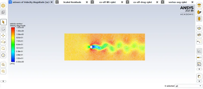
The animation for the simulation has been attached in the files section named as 'velocity-animation'

Ansys Fluent for Part-II (Re=10, 100, 1000, 10000, 100000)

The Fluent setting will be kept same as the first case of Part-I i.e. a steady state solver and the SIMPLE scheme method.

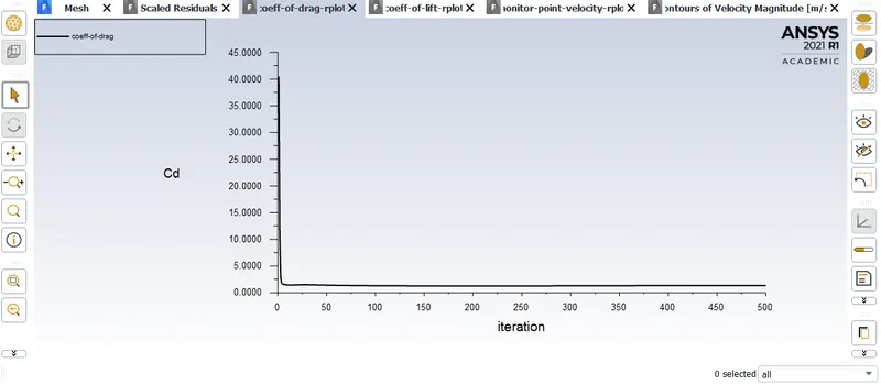
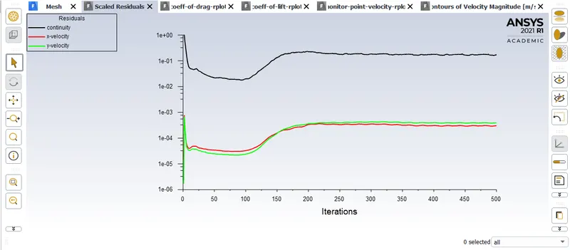
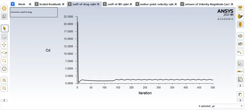
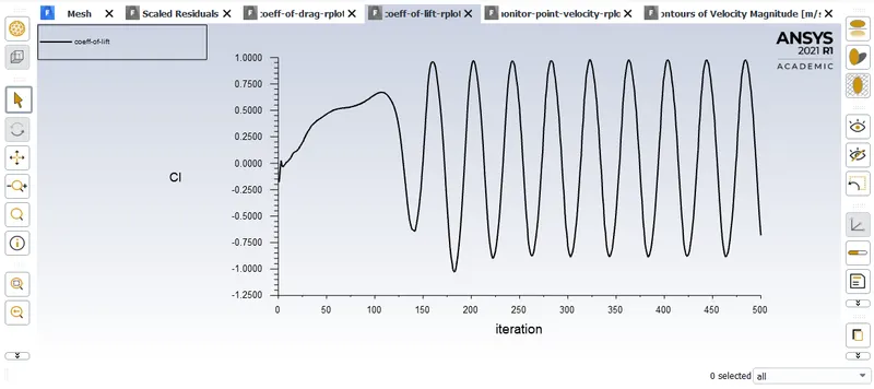
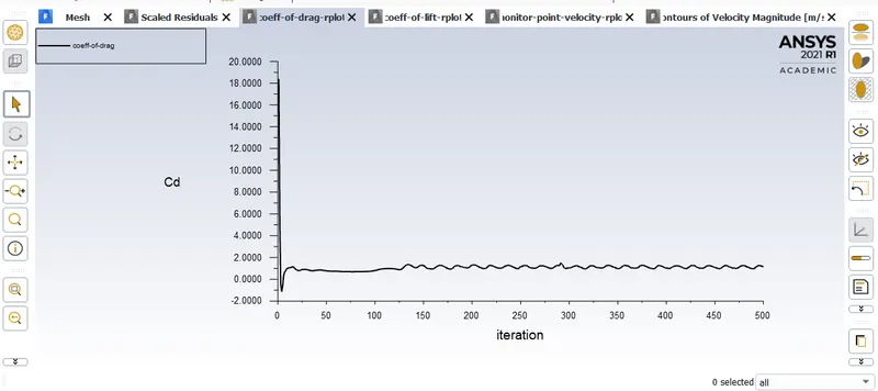
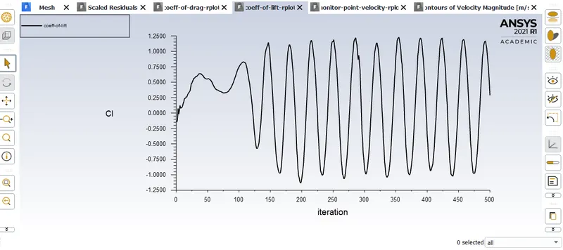
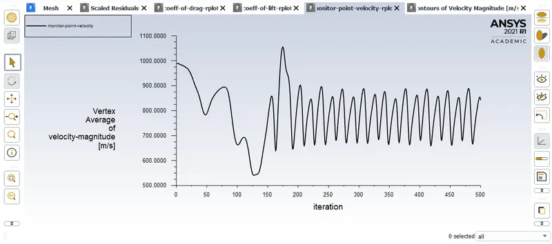
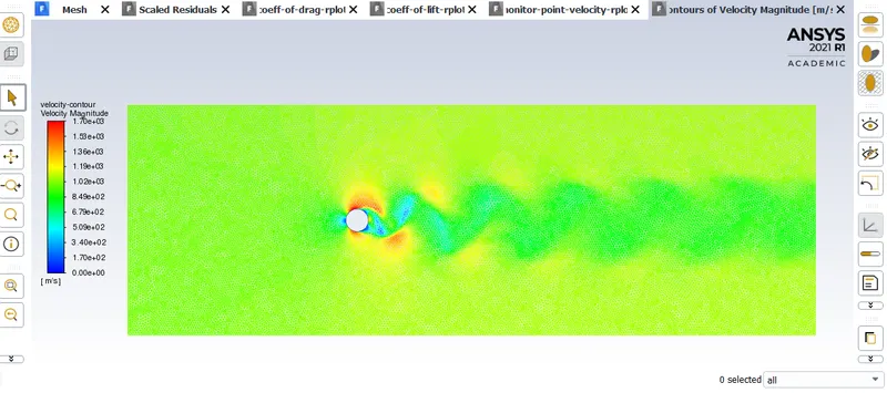
The values for the boundary condition at the inlet is calculated for every Reynolds number and substituted each time in the formula. The results for every case are displayed below sequentially. For every case the results will be in the order: Scaled residuals, Co-efficient of drag, Co-efficient of lift, Vertex average of velocity, Velocity contour.

Results-

1. Re = 10, ∴ u = 0.1 m/s

2. Re = 100, ∴ u = 1 m/s

3. Re = 1000, ∴ u = 10 m/s

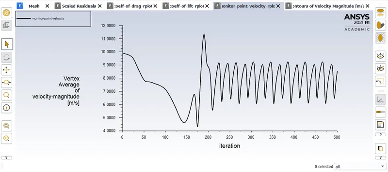
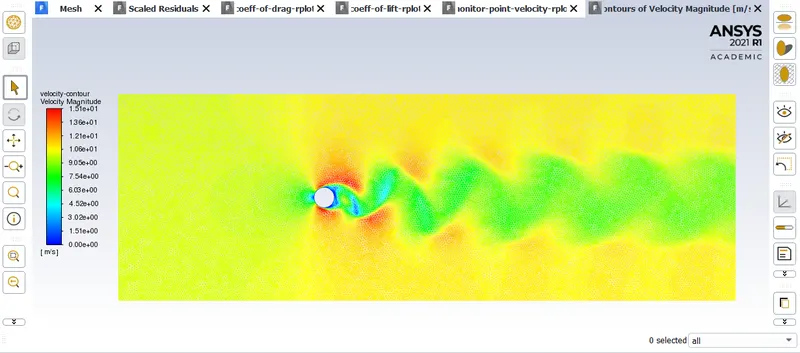
4. Re = 10000, ∴ u = 100 m/s

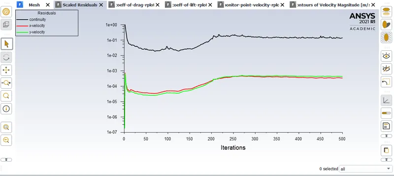
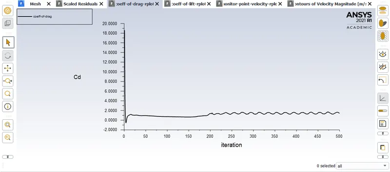
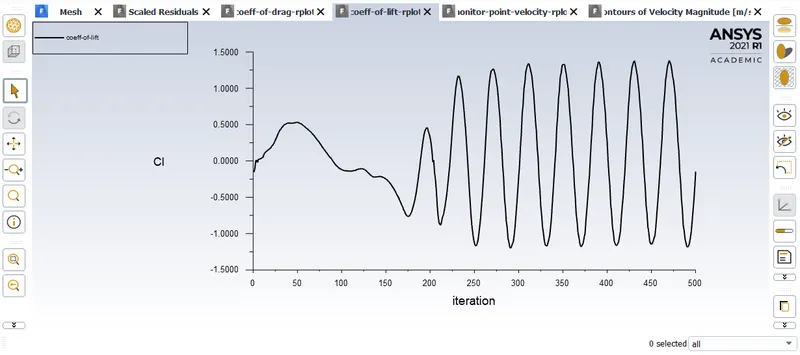
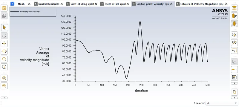
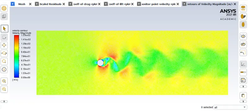
5. Re = 100000, ∴ u = 1000 m/s

Conclusion-

Since in all of the above graphs the line forms a certain pattern and stabilises and will continue forming the same pattern for further iterations, hence it can be inferred that all of the above solutions has surpassed convergence.

The values of the co-efficient of drag can be compared with its Reynolds number with the aid of a table.

Table 1-

Reynolds number (Re)	Co-effiecient of drag (Cd)
10	5
100	2
1000	1.25
10000	1.1
100000	1.05

The standard literature for reference.

Table 2-

Velocity (u)	Reynolds number (Re)	Co-efficient of drag (Cd)
0.1	10	3.355312
1	100	1.347501
10	1000	1.193902
100	10000	1.028611
1000	100000	0.953672

This standard literature is provided by the support engineer at Skill Lync.