Week 3 - Solving second order ODEs

Aim- To write a program that solves the following ODE.

Write a program in Matlab that will simulate the pendulum motion.

Theory-

A second order ordinary differential equation is an ordinary differential equation in which any derivatives with respect to the independent variable have order no greater than 2.

The general second order ODE can be written as:

 F(x, y, dy/dx, d^2 y/dx^2)

A simple pendulum can be described as a device where its point mass is attached to a light inextensible string and suspended from a fixed support. The vertical line passing through the fixed support is the mean position of a simple pendulum.

The equation of motion of a simple pendulum with damping-

where,

g = gravity in m/s2,

L = length of the pendulum in m,

m = mass of the ball in kg,

b = damping coefficient.

Coding-

1. Second order ODE code-

clear all
close all
clc

b=0.05;
g=9.81;
l=1;
m=1;

%initial conditions
theta_0 = [0;3];

%time points
t_span = linspace(0,20,500);

%solve ODE
[t, results] = ode45(@(t,theta) ode_func(t, theta, b, g, l, m), t_span, theta_0);

figure(1)
plot(t,results(:,1))
hold on
plot(t,results(:,2))
xlabel('time')
ylabel('plot')

%for animation
%counter 
ct = 1;
for i = 1:length(t)
    x0 = 0;
    y0 = 0;
    x1 = l*sin(results(i,1));
    y1 = -l*cos(results(i,1));

    figure(2)
    plot([x0 x1], [y0 y1], 'color', 'r')
    hold on 
    plot([1 -1], [0 0], 'color', 'b')

    plot(x1,y1, '.', 'MarkerSize', 50)
    axis([-2 2 -2 2])
    hold off

    M(ct) = getframe(gcf);
    ct = ct+1;
end

movie(M)
videofile = VideoWriter('Simple_Pendulum.avi','uncompressed AVI');
open(videofile)
writeVideo(videofile,M)
close(videofile)

2. ode_func code-

function [dtheta_dt] = ode_func(t, theta, b, g, l, m)

         theta1 = theta(1);
         theta2 = theta(2);
         dtheta1_dt = theta2;
         dtheta2_dt = -(b/m)*theta2 - (g/l)*sin(theta1);
         dtheta_dt = [dtheta1_dt ; dtheta2_dt];
end 

Explanation-

1. Second order ODE

• The initial conditions are defined which in this case 0 for the angular displacement and 3 for angular velocity.
• The timepoints are defined that is the number of values between the start and end of the pendulum motion, the 'linspace' command is used for 500 values between 0 and 20 (seconds).
• The ODE command is called in which has 't', 'results' as its output. The 'ode45' function is called in and the ode function, the time span and the initial points are put in. For the ode function, it is entirely defined in a different script which is defined in the second point.
• Plotting commands are called in and the time vs displacement and velocity are plotted.
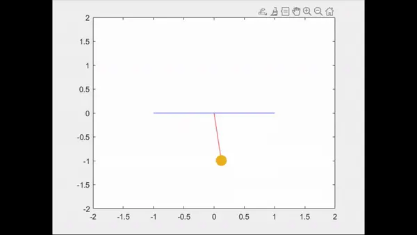
• The syntax for creating a movie of the animation is produced.

2. ode_func

• The function is defined with output as 'dtheta_dt' and the inputs to this function are 't', 'theta', 'b', 'g', 'l' and 'm'.
• The equations for 'theta1' and 'theta2' is defined along with its derivatives.

Results/Output/Animation-

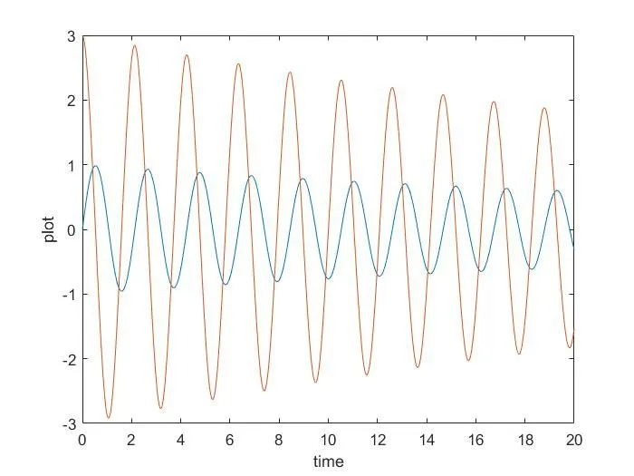
_____ Angular velocity

_____ Displacement

Errors encountered-

No complex errors occured while performing the entire program.

Except for a minor one where the minus sign for y1 coordinate was missing in the for loop which resulted in an inverted animation of the pendulum.