Challenge

Week 4.1 - Genetic Algorithm

FFurquan Acharwala30 Nov 2021

Aim - To write a code in MATLAB to optimise the stalagmite function and find the global maxima of the function.

Theory -

Genetic Algorithm -

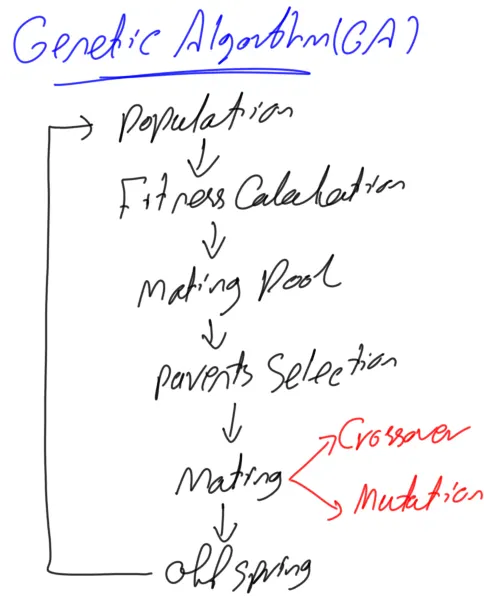
Genetic Algorithm (GA) is a search-based optimization technique based on the principles of Genetics and Natural Selection. It is frequently used to find optimal or near-optimal solutions. It is frequently used to solve optimization problems, in research, and in machine learning.

GA is based on Darwin’s theory of evolution. It is a slow gradual process that works by making changes to the making slight and slow changes. Also, GA makes slight changes to its solutions slowly until getting the best solution.

GA works on a population consisting of some solutions where the population size (popsize) is the number of solutions. Each solution is called individual. Each individual solution has a chromosome. The chromosome is represented as a set of parameters (features) that defines the individual. Each chromosome has a set of genes. Each gene is represented by somehow such as being represented as a string of 0s and 1s.

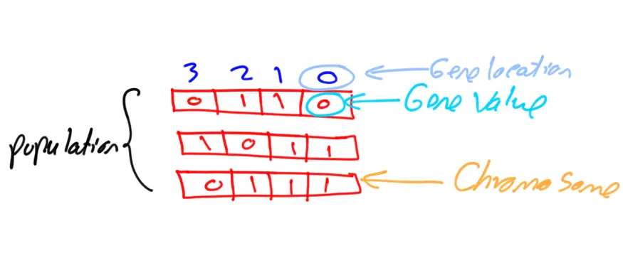
Also, each individual has a fitness value. To select the best individuals, a fitness function is used. The result of the fitness function is the fitness value representing the quality of the solution. The higher the fitness value the higher the quality the solution. Selection of the best individuals based on their quality is applied to generate what is called a mating pool where the higher quality individual has higher probability of being selected in the mating pool.

The individuals in the mating pool are called parents. Every two parents selected from the mating pool will generate two offspring (children). By just mating high-quality individuals, it is expected to get a better quality offspring than its parents. This will kill the bad individuals from generating more bad individuals. By keeping selecting and mating high-quality individuals, there will be higher chances to just keep good properties of the individuals and leave out bad ones. Finally, this will end up with the desired optimal or acceptable solution.

But the offspring currently generated using the selected parents just have the characteristics of its parents and no more without changes. There is no new added to it and thus the same drawbacks in its parents will actually exist in the new offspring. To overcome such problem, some changes will be applied to each offspring to create new individuals. The set of all newly generated individuals will be the new population that replaces the previously used old population. Each population created is called a generation. The process of replacing the old population by the new one is called replacement.

Optimization -

Optimization is a decision making process, it helps to find the best results under a set of prioritized criteria or constraints. It is a procedure which is executed iteratively by comparing various solutions till an optimum or a satisfactory solution is found.

Optimization methods are used in many areas of study to find solutions that maximize or minimize some study parameters, such as minimize costs in the production of a good or service, maximize profits, minimize raw material in the development of a good, or maximize production.

An optimization algorithm is a procedure which is executed iteratively by comparing various solutions till an optimum or a satisfactory solution is found. With the advent of computers, optimization has become a part of computer-aided design activities.

Stalagmite function-

A stalagmite is an upward-growing mound of mineral deposits that have precipitated from water dripping onto the floor of a cave. Most stalagmites have rounded or flattened tips. There are many other types of mineral formations found in caves.

In MATLAB, a stalagmite function generally refers to the function with which we are generating values over a stalagmite kind of surface for finding out the local and global maxima and minima of that particular given function.

Coding and explanation -

clear all
close all
clc

%Defining our searchspace
x = linspace(0,0.6,150);
y = linspace(0,0.6,150);
num_spaces = 50;

%creating a 2dimensional mesh
[xx, yy] = meshgrid(x,y);

for i = 1:length(x)
    for j = 1:length(y)
        input_vector(1) = xx(i,j);
        input_vector(2) = yy(i,j);
        f(i,j) = stalagmite(input_vector);
    end
end

In this block of code the searchspace is defined with 150 values in x and y each.
The 'num_spaces' is used to define the number of iterations i.e. 50 in this case.
A two dimensional mesh is defined using the 'meshgrid' command.
A 'for loop' is generated which defines 'i' and 'j'. For every value of 'i' the entire 'j' array is assigned to it, which gives us coordinates for the input vector (1) and (2) whose values are then given to the stalagmite function after which we obtain the coordinates of the z-value i.e. f(i,j).

%Study 1 - unbounded 
tic
for i = 1:num_spaces
    [results,fopt(i)] = ga(@stalagmite,2);
    xopt(i)=results(1);
    yopt(i)=results(2);
end
study_time_1 = toc

figure(1)
subplot(2,1,1)
surf(x,y,-f)
shading interp 
hold on
plot3(xopt,yopt,-fopt,'marker','o')
subplot(2,1,2)
plot(-fopt)
xlabel('iteration')
ylabel('function maximum')

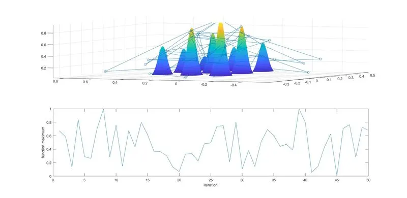
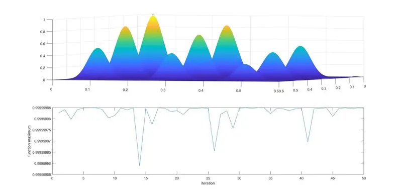
In this study the limit for generating the values have not been set. This means the optimum values could be generated above and beyond 0.6, since we have not defined in the script for 0.6 to be the threshold value.
The plots are generated and the study time is calculated using the 'tic' and 'toc' command. It took 4.4289 seconds for this case, which is quick given the num_spaces = 50.
In the 'for loop' the genetic algorithm function is plugged in and for every iteration the x,y and z values are recorded.
The surface plot and the 2D plots are obtained using the subplot command.
'-fopt' will give us the global maxima values since the algorithm by default gives the minima values.

%Study 2 - bounded
tic
for i = 1:num_spaces
    [results,fopt(i)] = ga(@stalagmite,2,[],[],[],[],[0;0],[0.6;0.6]);
    xopt(i) = results(1);
    yopt(i) = results(2);
end
study_time_2 = toc
figure(2)
subplot(2,1,1)
surf(x,y,-f)
shading interp
hold on
plot3(xopt,yopt,-fopt,'marker','o')
subplot(2,1,2)
plot(-fopt)
xlabel('iteration')
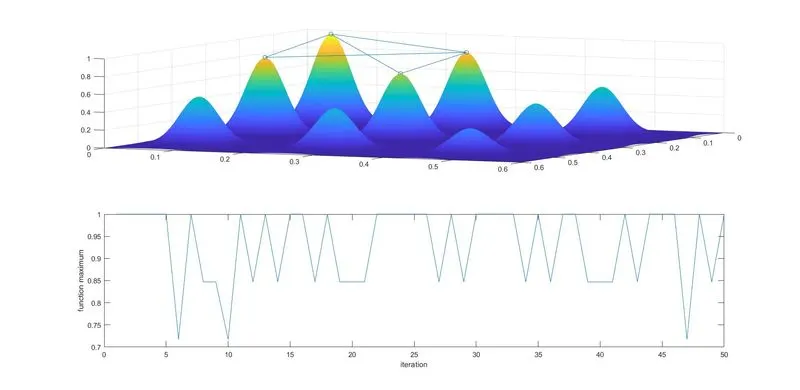
ylabel('function maximum')

The limits for the values are given and is bounded between 0 and 0.6 using the commands in the GA function from the video.
The study time for this case was 5.2720 seconds which is hardly a second longer than the previous case.

% Study 3 - increased initial population

tic
options = optimoptions('ga');
options = optimoptions(options,'populationsize',250);
for i = 1:num_spaces
    [results,fopt(i)] = ga(@stalagmite,2,[],[],[],[],[0;0],[0.6;0.6],[],[],options);
    xopt(i) = results(1);
    yopt(i) = results(2);
end
study_time_3 = toc

figure(3)
subplot(2,1,1)
surf(x,y,-f)
shading interp
hold on
plot3(xopt,yopt,-fopt,'marker','o')
subplot(2,1,2)
plot(-fopt)
xlabel('iteration')
ylabel('function maximum')

The initial population size in this case has been defined as 250 using the 'optimoptions' command.
The study time for this case is 15.3720 seconds.

The stalagmite function code -

function A = stalagmite(input_vector)
x=input_vector(1);
y=input_vector(2);
f1 = (sin(5.1*pi*x+0.5)).^6;
f2 = exp ((-4*log(2)*((x-0.0667).^2))/0.64);
f3 = (sin(5.1*pi*y+0.5)).^6;
f4 = exp((-4*log(2)*((y-0.0667).^2))/0.64);
A = -(f1*f2*f3*f4);
end