Week 6 - CHT Analysis on a Graphics card

Aim- 1. To simulate CHT on a graphics card.

2. To check the temperature distribution on the graphics card and advise appropriate construction to avoid overheating.

Introduction-

Conjugate Heat Transfer Analysis or CHT analysis is done in a domain where a combination of modes of heat transfer takes place, where in this case it is convection and conduction. This type of analysis is done in a set up where heat transfer takes place between a solid and liquid sharing a common interface.

In this set up the fluid is air flowing over a graphics card which is a solid made of combination of materials.

Theory-

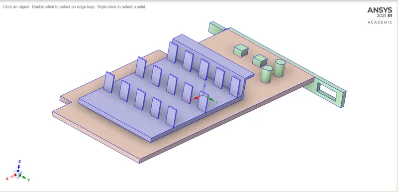
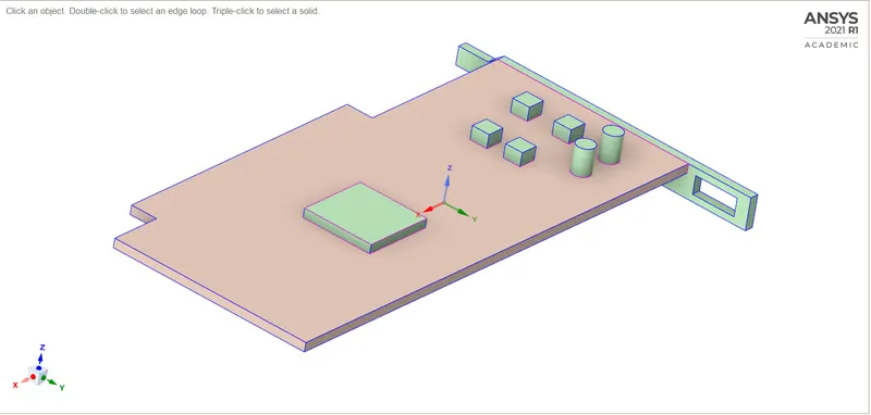
The graphics card is made of three components, the PCB, processor and the fins.

1. PCB material<Ref1> is made up of FR4 epoxy laminate and prepgreg in most part of the world. Since the Fluent database does not have this material it has to be defined as a user defined material in the database with the properties,<Ref2>

Density = 1850 kg/m^3

Thermal conductivity = 0.29 W/m.K

Specific heat capacity = 950 KJ/kg.K

2.The processor <Ref3> is made out of silicon, however, it is not used in its pure form but for the sake of simplicity we can use pure silicon for our simulation, properties of which are, <Ref4>

Density = 2000 kg/m^3

Thermal conductivity = 150 W/m.K

Specific heat capacity = 710 KJ/kg.K

3. The fins are typically made out of aluminium because of its good heat conductivity that it absorbs all the heat from the processor in its larger surface area and exposes to the air for rapid cooling. Aluminium is available in the fluent database.

4. The entire geomtery is exposed to air flow with its regular properties at 1m/s initially to 5m/s eventually. Air is available in the Fluent database.

5.The air velocity at inlet is assumed initially as 1.5 m/s and then increased to 5 m/s in two steps, giving us three cases.

6.In a regular graphic card the processor produces around <Ref5>, 75W of energy out of which 99.99% is absorbed by the processor and given out as heat also the remaining 0.01% energy is used to actually display the output on your monitor. The heat generation above is for a processor of dimensions 40x40x2 mm, so accordingly, 75/0.04x0.04x0.002 = 23437500 W/m^3 = 2.34375e+07 W/m^3. We can keep this value of heat generation for our processor which has a different dimension than the actual to make sure the appropriate temperatures are reached in the simulation.

Solving and modelling approach-

The geometry of the graphics card will remain the same for all the three cases. It will be articulated well just for the first case.

As we proceed with the cases the velocity of the air entering at the inlet which in real life is the air blown by the CPU fan.

The results will be compared such as the velocity contours, temperature contours to check the potential hotspots in the graphic card.

Every case will be run with a refined mesh quality. To identify what areas needs a better meshing a base line mesh will be run for the purpose.

Pre-processing and solver setting-

Geometry-

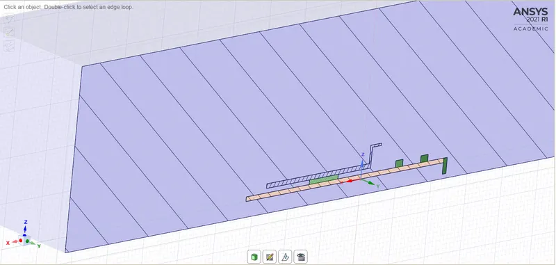
The geometry is ready with the graphic card and an enclosure for fluid flow.

Share topology is used to achieve conformal mesh.

Interference in the geometry is checked with the help of a function with the same name in Repair.

Mesh-

Named selections are made accordingly as inlet, outlet, symmetry and wall.

Since we are having a base-line set up initially, the mesh is generated with the default settings and without any refinement efforts. It is then updated in fluent.

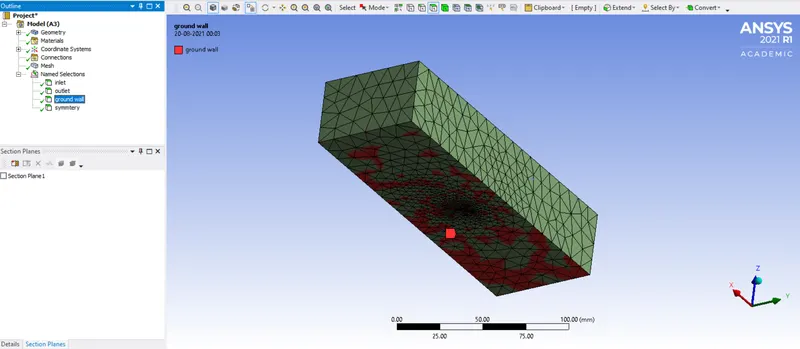
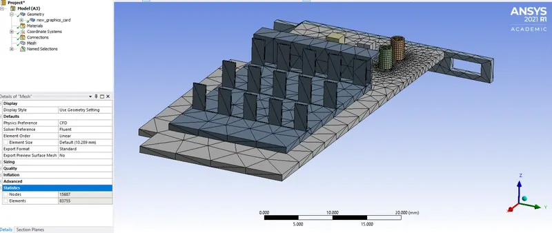
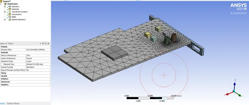
Number of elements = 83755

Element size = 10.289mm(default)

Fluent-

The steps to solve the equations for graphic card are-

1. Load or upload the geometry in fluent
2. Perform a mesh check to ensure no mesh errors.
3. Select the pressure based solver and absolute velocity formulation
4. This simulation is ran with a steady state solver.
5. Select the viscous model opting for k-epsilon Realizable model.
6. Create the necessary materials corresponding to the various components of the graphic card explained in Theory.
7. Assign the components as either solid or fluid, fluid being the enclosure and the rest of the components being solid.
8. Set the boundary conditions such as the velocity inlet magnitude as 1.5m/s.
9. Initialize the set up using hybrid initialization method.
10. Uncheck convergence in the Residuals option so that the model keeps simulating even after the solution has converged.
11. Hit calculation with 500 iterations and observe the residuals plot.

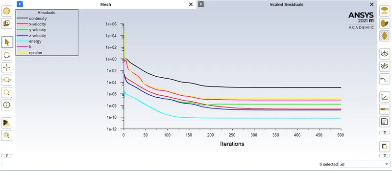
The solution converged at around 350 iterations.

Results-

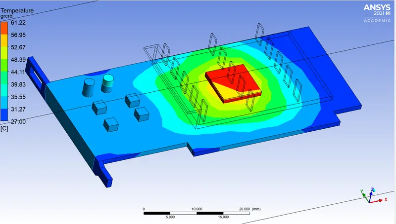
Temperature contour (local) -

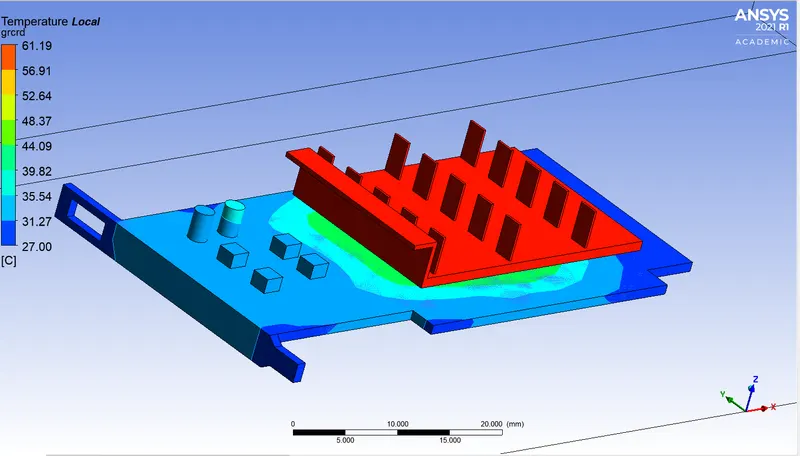
Temperature contour (global) -

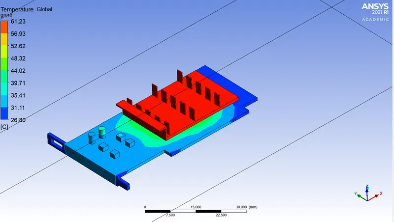
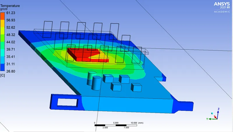
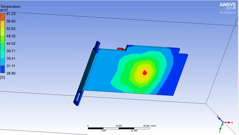
The global and local scale show no significant difference in their extreme values.

The potential hotspots are near the processor which happens to be our heat source, and requires a refined mesh.

On the base of the graphic card at the lower side the temperature distribution is very coarse, hence the base too will require a refined mesh.

The fins have a consistent distribution which prompts that the process did not capture the details of the temperature variations, so a refined mesh will solve this issue.

Refined set up with 1.5 m/s inlet velocity-

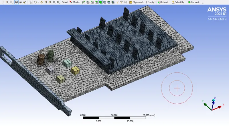
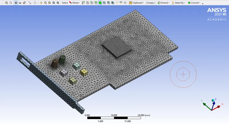
The geometry will remain unchanged and is not edited so the same geomtery can be used without opening the Spaceclaim module. The Mesh module is booted and the following refinements are made-

1. General element size = 5mm (enclosure)
2. Body sizing for Base = 0.8mm, Capture curvature = yes (18 deg)
3. Body sizing for processor = 0.4mm
4. Body sizing for fins = 0.4mm

Number of elements = 419556

Fluent-

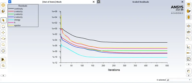
The solution has converged at around 325 iterations.

Results-

Temperature contour-

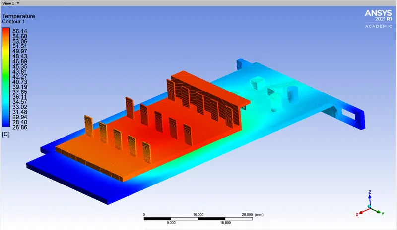
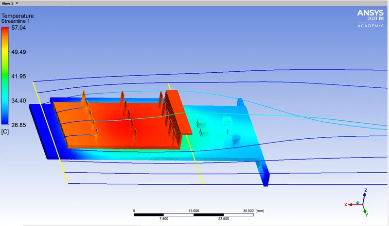
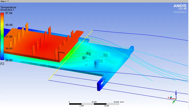
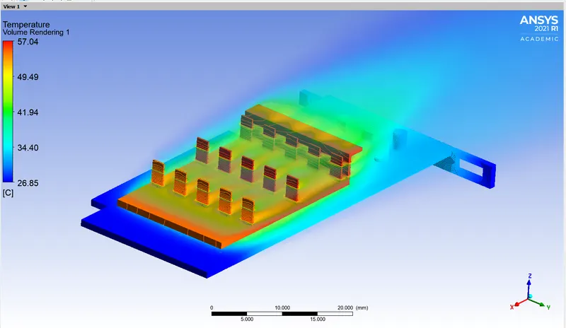
From the front part of the fins it is visible that the fins have started to cool by the air flow from 56C i.e. the highest temperature on scale to around 52C.

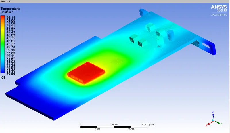
The base at the back has absorbed a bit of the heat to around 43C.

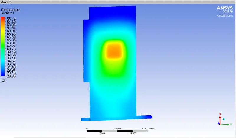
The part of the base attached to the processor has a temperature of around 53C.

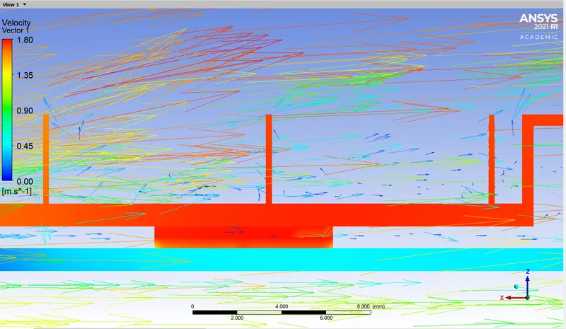
Velocity vectors-

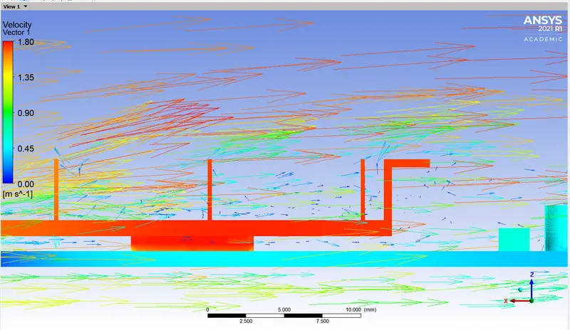
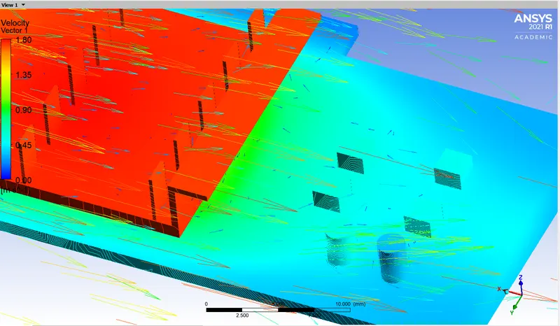
The velocity vectors show areas of the recirculation region formed behind the fins due to air flowing over it. This velocity is almost near to being 0m/s.

Temperature streamlines-

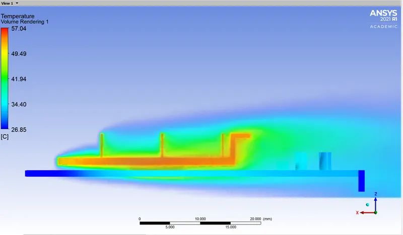
Temperature volume rendering-

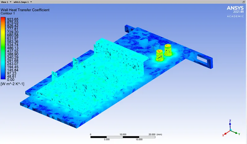
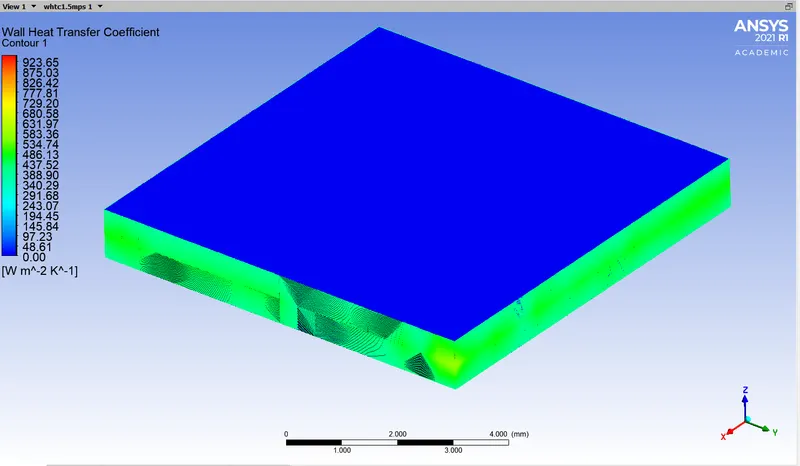
Wall heat transfer coefficient-

Refined set up with 3m/s air velocity-

The geometry and Mesh will remain unchanged with the same meshing refinements made in the previous case.

As for Fluent the boundary condition at the inlet velocity has to be changed with the magnitude of velocity as 3m/s.

Residuals plot-

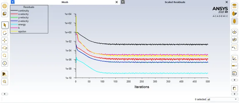
The solution has converged at around 150 iterations.

Results-

Temperature contour-

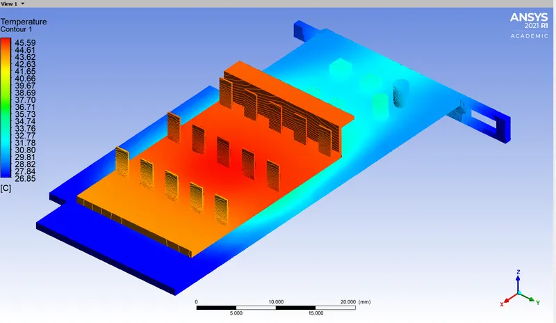
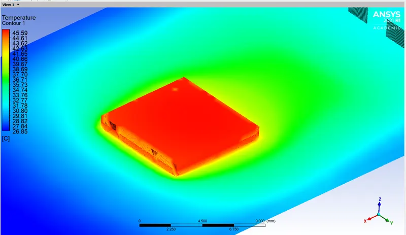
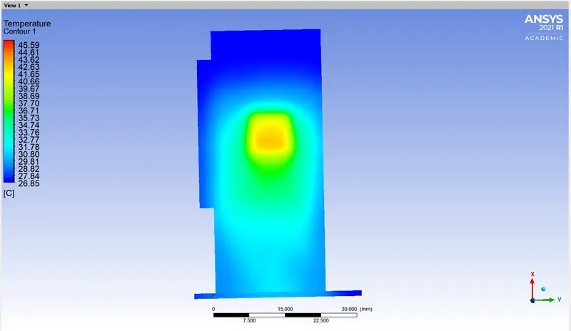
Velocity vectors-

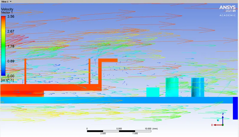
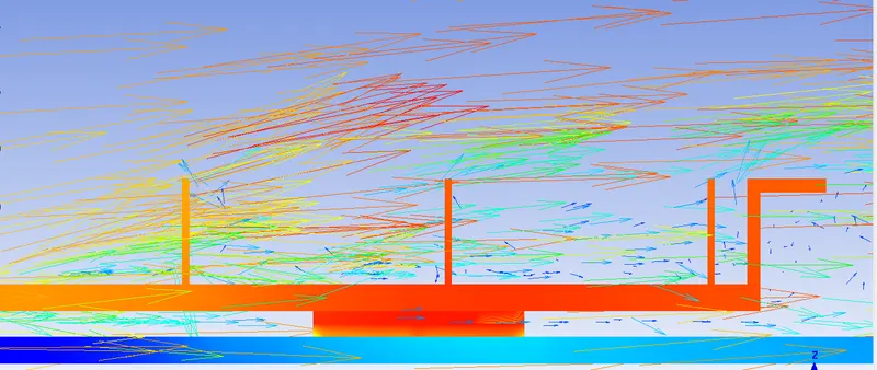
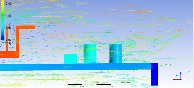
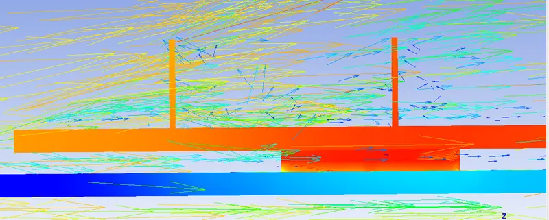
The vectors for the velocity are behaving in an appropriate manner with the recirculation region forming behind every fin and also at the back of the entire fin structure.

Temperature streamlines-

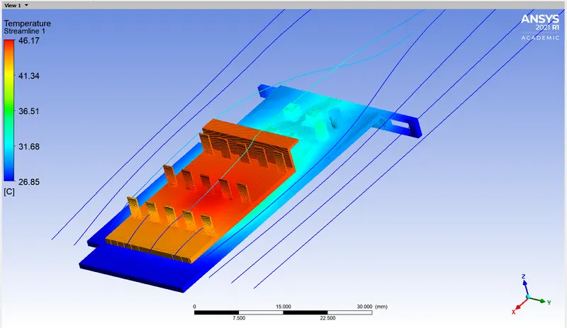
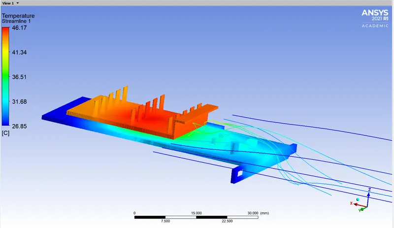
Temperature volume rendering-

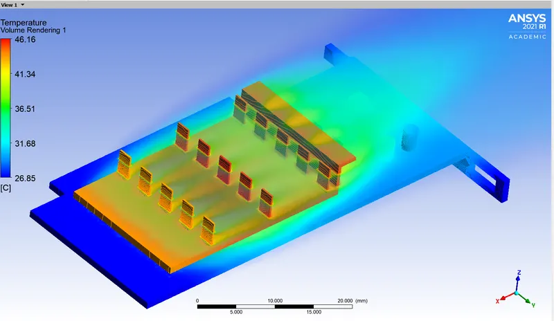
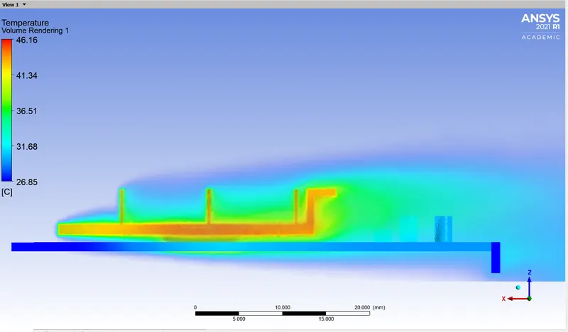
By this excellent visuals over the temperature distribution over the solid as well as the fluid component the fin has significantly cooled down to around 42C.

Wall heat transfer coefficient-

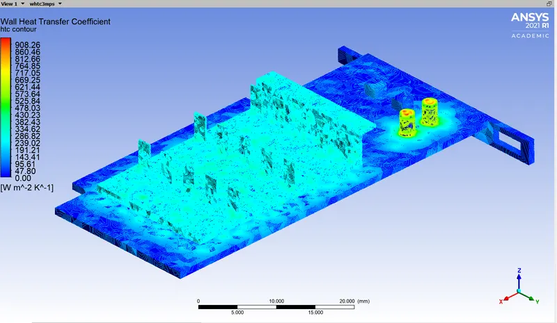
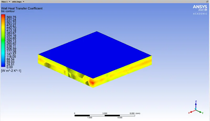
The HTC for the processor is around 442W/m^2.K

Refined set up with 5 m/s inlet velocity-

The geomtery and mesh remains unchanged. The boundary condition at inlet has to be changed to the velocity magnitude of 5m/s.

Residuals plot-

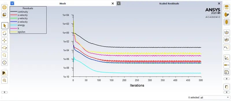
The solution has converged at around 225 iterations.

Results-

Temperature contour

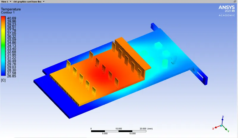
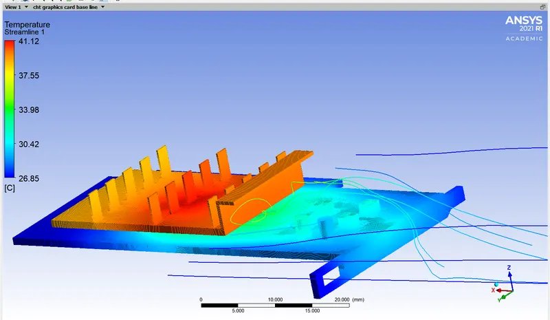
The front part of the fins has significantly cooled down with the increase in air velocity to around 39C.

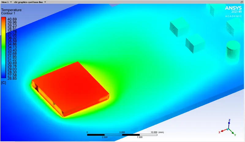
The air velocity has been increases to an extent where it is directly trying to cool the processor as seen in the front face of the processor the temperature is around 38C.

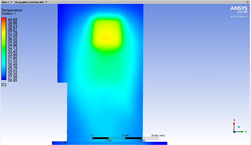
The lower part of the base has also lost a lot of temperature and this hotspot is at around 37C.

Velocity vector-

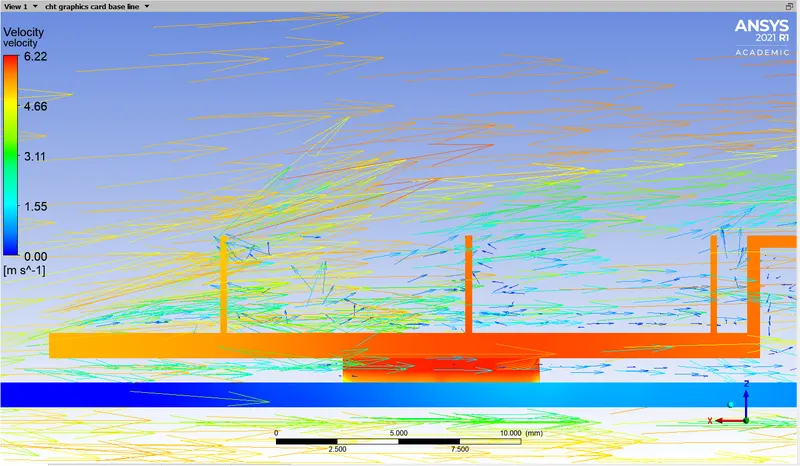
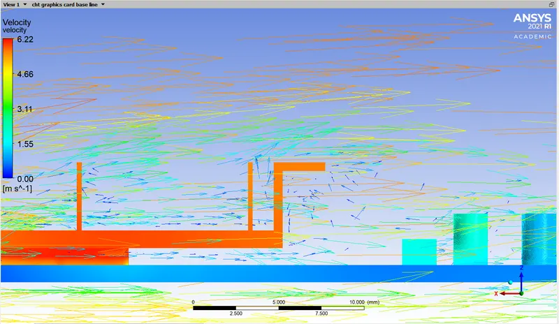
The velocity vectors show the direction and magnitude of the air flowing, the recirculation region being formed behind the fin walls.

Temperature streamline-

Wall heat transfer coefficient-

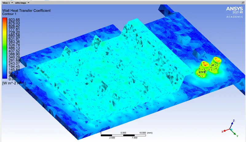
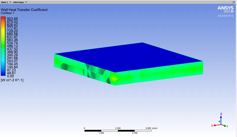
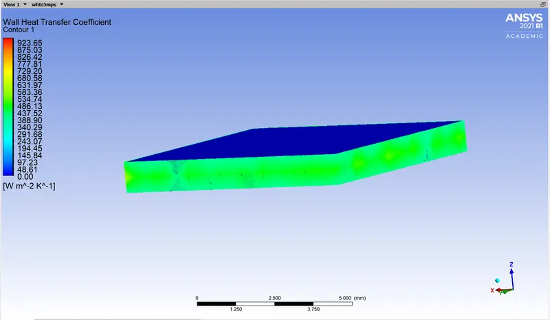
The HTC for the processor is around 500W/m^2.K

Conclusion-

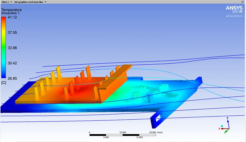
With the increase in air velocity the temperature on the fins decreases significantly on the front side which leads to heat transfer from the processor to the fins through conduction and later to the air through convection, a proper conjugate heat transfer process taking place.

For the potential hotspots the area below the processor on the lower part of the base is a hotspot where attaching other components of the system should be avoided since it may hinder the air flow over the spot consequently rising the temperatures. Leaving the entire lower face of the base is advisable so that maximum air flow comes in contact with the area.

The potential hotspot of the graphic card-