Week - 8 Mass Scaling

Week 8 Mass Scaling

AIM:

1. To use mass scaling to reduce the runtime of a model and ensure the stability of mass scaling.
2. To reduce the runtime required to run the analysis of the given model using mass scaling technique and stability has to be completely intact.
3. To plot a histogram to compare the runtime with mass scaling trials.
4. To optimize both the DT and TSSFAC parameters.
5. To run the same model using implicit solver with necessary changes and compare implicit and explicit runtime

Note: The limit on mass scaling is 8%.

INTRODUCTION:

1. Mass-scaling is a term that is used for the process of scaling the element’s mass in explicit simulations to adjust its timestep. The primary motivation is to change the global compute timestep which is limited by the Courant’s stability criteria.

1. LS-DYNA allows two different types of mass-scaling using the DT2MS parameter from *CONTROL_TIMESTEP with the default set to no mass-scaling.

1. When DT2MS is less than zero, LS-DYNA adds mass of each element whose timestep is below abs (DT2MS) such that the element’s updated DT is equal to abs (DT2MS).

1. When DT2MS is greater than zero, LS-DYNA adds mass to elements whose DT is below abs (DT2MS) and “removes” mass from elements whose DT is greater than zero.

1. DT2MS>0 is seldom used while DTM2<0 is frequently used for overcoming the smallest computed timestep.

1. Care must be taken when using DT2MS<0 to ensure that the added mass does not have an adverse effect on the simulation accuracy. It is common practice to limit the percentage of added mass to less than 5% (at part level) in dynamic simulations.LS-DYNA outputs the percentage of added mass at component level which is a better indicator of amount of added mass due to mass-scaling.

7. Mass-scaling refers to a technique whereby nonphysical mass is added to a structure in order to achieve a larger explicit timestep. The runtime of FE simulation is mainly a function of a model size and size of the solution step. As the size of the model is not in our control, we must play with varying timestep. Thus, bigger the timestep, faster the simulation is. But fixing the range of bigger timestep, depends on the sensitivity of the model and accuracy required.

As per Courant-Friedrichs condition for explicit analysis is.

Where,

Delta t is the timestep,

E min = size of the smallest mesh element,

c = Speed of the stress/shear wave

The scaling factor is used for providing numerical stability to the solution.

Also,

E = Young’s Modulus

rho= Density

If we increase the density of a small element, we get an increased timestep.

So, solution run time will reduce.

8. LS-DYNA allows two different types of mass-scaling using the DT2MS parameter from *CONTROL_TIMESTEP with the default set to no mass scaling. When DT2MS is less than zero, LS-DYNA adds mass of each element whose timestep is below abs (DT2MS) such that the element’s updated DT is equal to abs (DT2MS). When DT2MS is greater than zero, LS-DYNA adds mass to elements whose DT is below abs (DT2MS) and “removes” mass from elements whose DT is greater than zero. DT2MS>0 is seldom used while DTM2S.

Here, the simulation is carried out initially without Mass scaling to find default computational time and then by varying the mass scaling parameters to reduce computational or simulation time.

PROCEDURE:

In this project, the runtime has to be reduced using mass scaling technique by varying the values of DT2MS and TSSFAC with percentage increase of mass within 8% using Explicit and Implicit analysis.

Without Mass scaling:

Initially the simulation is set to run without mass scaling parameters.

So, the default computational time can be observed with LS-Dyna manager as given blow:

if we activate *Control Timestep keyword, and do not add any mass or without any adding mass scaling parameters changes, the computational time will be as given below:

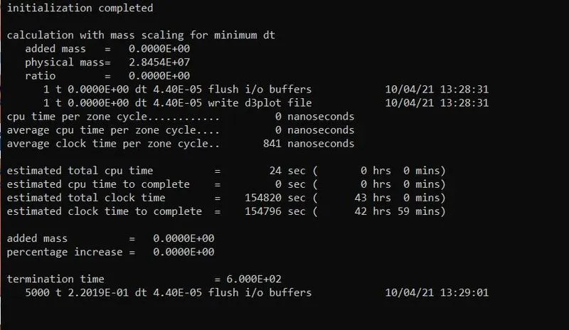
• Here we can see that there is also a huge time up to 42 hrs 59 mins.

Explicit Analysis

• Here we will see first the explicit method for mass scaling with variable timestep and constant timestep sale factor.

Mass scaling with variable timestep and constant TSSFAC = 0.9

• Here we have kept the value of TSSFAC = 0.9 constant and only the timestep value is changing in below manner.

Timestep/ DT2MS = 5.5E-5:

• Here we have activated *Control Timestep keyword and set DT2MS/ Timestep = -5.5E-5 and kept TSSFAC = 0.9

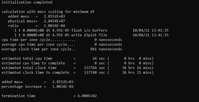
• Here we can see that we have added the mass up to 2.8552E+03 which is 0.01%.
• We can observe that computational time has been decreased up to 38 hrs. 15 mins

Timestep/ DT2MS = 6.5E-5:

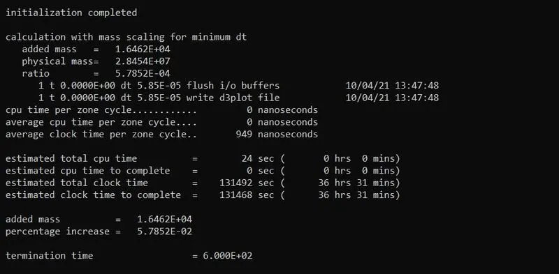
• Here we can see that we have added the mass up to 1.6462E+04 which is 0.0578%.
• We can observe that computational time has been decreased up to 36 hrs. 31 mins.

Timestep/ DT2MS = 7.5E-5:

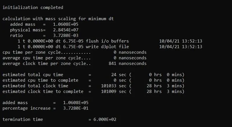
• Here we can see that we have added the mass up to 1.0608E+05 which is 0.37%.
• We can observe that computational time has been decreased up to 28 hrs. 3 mins.

Timestep/ DT2MS = 8.5E-5:

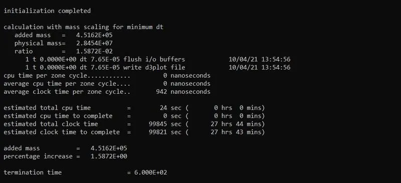
• Here we can see that we have added the mass up to 4.5162+05 which is 1.58%.
• We can observe that computational time has been decreased up to 27 hrs. 43 mins.

Timestep/ DT2MS = 9.5E-5:

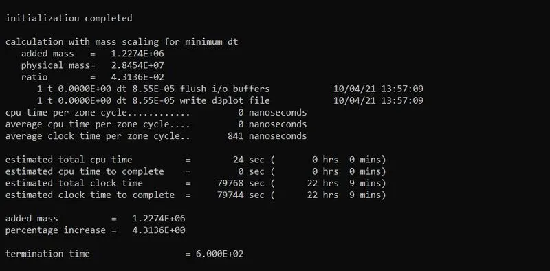
• Here we can see that we have added the mass up to 1.2274+06 which is 4.31%.
• We can observe that computational time has been decreased up to 22 hrs. 9 mins.

Timestep/ DT2MS = 10E-5:

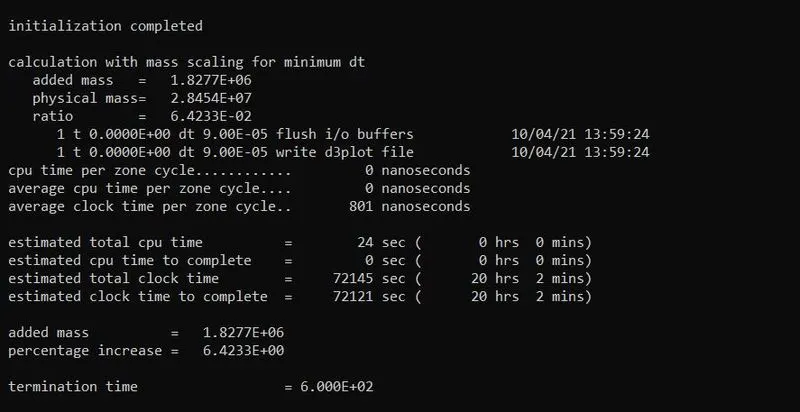
• Here we can see that we have added the mass up to 1.8277+06 which is 6.42%.
• We can observe that computational time has been decreased up to 20 hrs. 02 mins.

Timestep/ DT2MS = 10.3E-5:

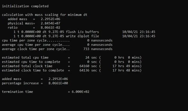
• Here we can see that we have added the mass up to 2.2952+06 which is 8.06%.
• We can observe that computational time has been decreased up to 17 hrs. 48 mins.

Here we have reached up to 8 % limit of the mass scaling, so we should not add further mass.

Mass scaling with Constant timestep and variable TSSFAC = 0.9

• Since we have reached up to 8% of added mass and got the minimum computational timestep, so now we will fix that timestep and with that constant timestep, we will observe the effect of changing the values of TSSFAC (Timestep scale factor).
• As the minimum TSSFAC limit should be 0.6, we will change that up to only 0.6.

TSSFAC = 0.9 , DT2MS = 10.3E-5:

• We can observe that computational time is minimum up to 17 hrs. 48 mins.

TSSFAC = 0.8, DT2MS = 10.3E-5:

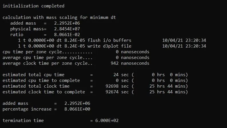
• We can see that computational time is increased up to 25 hrs. 44 mins.
• Here the percentage increase in added mass is constant at 8.06.

TSSFAC = 0.7, DT2MS = 10.3E-5:

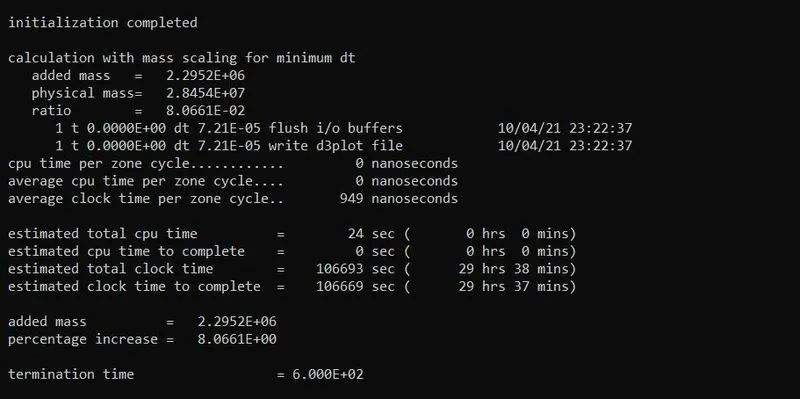
• We can see that computational time is increasedmore up to 29 hrs. 38 mins.

TSSFAC = 0.6, DT2MS = 10.3E-5:

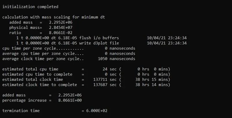
• We can see that computational time is increasedmore up to 38 hrs. 14 mins.

• As we have reached up to minimum TSSFAC value = 0.6, and we can observe the increase in computational time with decrease in Timestep scale factor.

Implicit Analysis

Here the same simulation is set to run with Implicit method.

To activate or use the Implicit method, with same content of Keywords, we must add or change in some Keywords.

Follow the below procedure for running the simulation with Implicit method:

• Use “*Control Implicit General” card. To activate implicit method, set IMFLAG = 1.
• Keep initial timestep/ DT0 = 1.
• Use “*Control Implicit Auto” card. For auto adjustment of timestep size, keep IAUTO = 1.
• Use “Control Implicit Solution” card, so that system can choose the analysis type between linear and non-linear.
• Use “*Control Implicit Solver” card, where stiffness matrix invention takes place. Keep LSOLVER = 4, to run the simulation with single precision to save run time compared to double precision.

On using different keywords, and with Implicit method, the computational time is calculated as below:

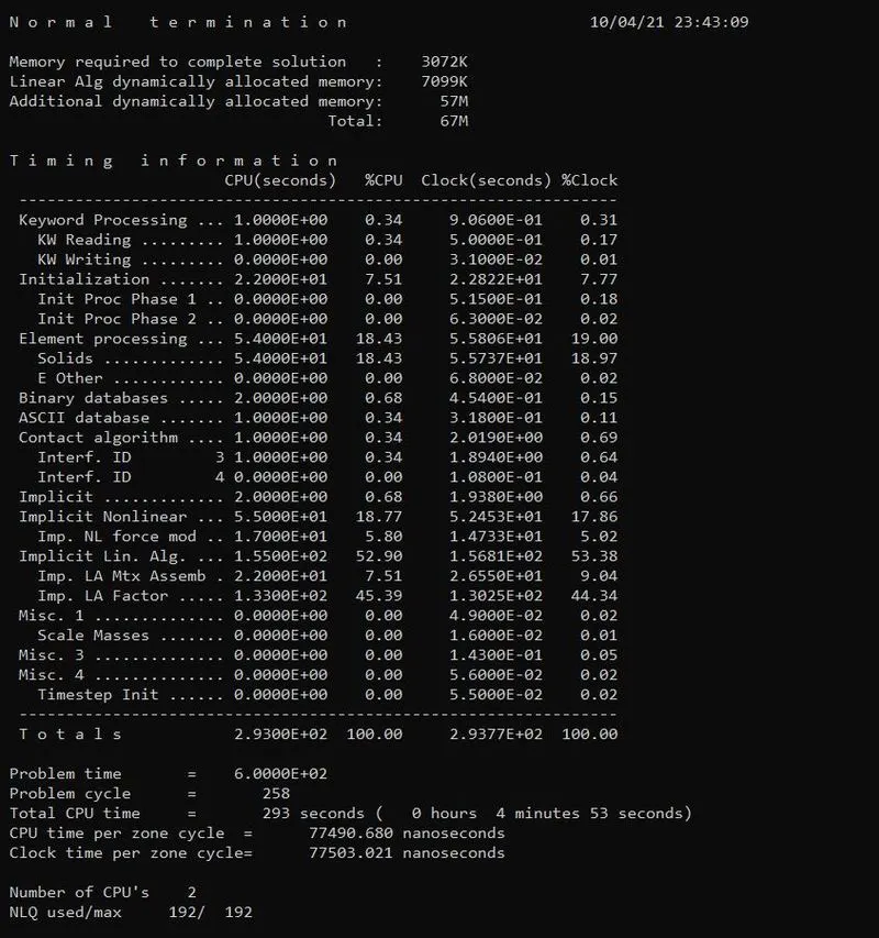
• As shown in above image, we can observe that implicit method takes the least time up to 4 min. 53 secs.
• This shorter time is because of initial timestep = 1, which is used with constant timestep formulation and termination time is large.
• The timestep in implicit analysis is well considered and this method is good in terms of accuracy.

Comparison:

Comparison of Run Time for Mass scaling with Variable Timestep and constant Timestep scale factor iun explicit analysis :

Since we have done many trials on mass scaling up to 8% limit and got the reduced computational time.

Now we can observe the data from the results and compare the computational time with change in Timestep and constant Timestep scale factor as below:

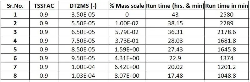
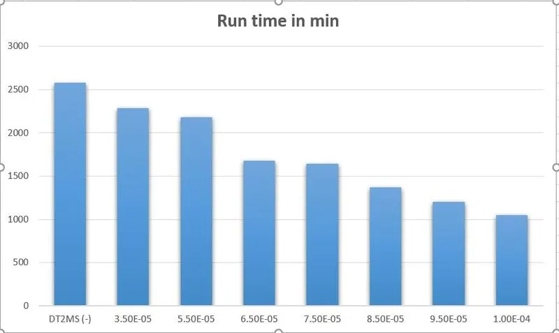
• From above tabular data and histogram, we can observe that as we increase the timestep value, added mass or mass scaling percentage increase and the computational time decreases.
• We can observe that least computational time is achieved at 8 % mass scaling up to 17.48 hrs. or 1048 Mins.

Comparison of Run Time for Mass scaling with Constant Timestep and Variable Timestep scale factor in explicit analysis:

• After reaching the limit of 8% mass scaling, we can also check the effect of change in timestep scale factor by changing TSSFAC value.
• So, with change in TSSFAC, change in Computational time can be describes as below:

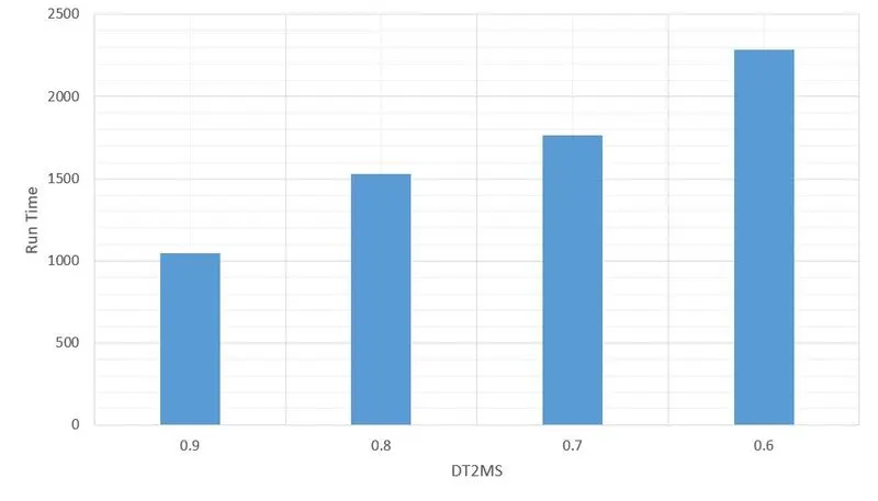
• From above tabular data and histogram, we can observe that as we decrease the timestep scale factor value, with constant added mass or mass scaling percentage, the computational time increases.
• We can observe that least computational time is achieved at 8 % mass scaling up to 17:48 hrs. or 1048 Mins with TSSFAC / Timestep scale factor = 0.9.
• From TSSFAC = 0.9 to TSSFAC = 0.6, computational time increases.

Comparison of Run Time between Explicit and Implicit Analysis:

• From above study we can compare the results between explicit and implicit analysis.
• We can observe that as we add the mass or increase the mass scaling percentage, we can reduce the computational time.
• From the Time step scale factor change, we can observe that as the Timestep scale factor TSSFAC increases, Computational time decreases.
• By optimizing the value of Timestep scale factor (TSSFAC) and Timestep (DT2MS), we have achieved the least computational time up to 17 hrs. 38 mins.
• But also, we can observe that if we use the Implicit method for running the same simulation, we can reduce the computational time to very low up to 4 min 53 sec.
• So, by comparing the implicit and explicit methods, we can get very least computational time with accuracy and with stable model in case of implicit method.

Conclusion:

• From the study, we can conclude that in explicit method, we can reduce the solution time with help of mass scaling.
• We can observe that in explicit method, by decrease in TSSFAC from 0.9 to 0.6, actual timestep decreases due to decreased scale factor and results in high computational time.
• But if we keep TSSFAC to 0.9 and increase the Mass scaling percentage or add the mass up to 8%, we can observe decrease in computational time in a significant way.
• Limit of 8% mass scaling is because of stability of the model. As we increase too much mass, then the inertia will be added to the model and the model can be unstable.
• Thus, for explicit method, Mass scaling is very helpful to reduce the computational time for very large simulations.
• In implicit method, we can put the values of DTMAX and DTMIN with DTO (Initial timestep). But by giving IAUTO = 1, we are allowing the system to adjust the timestep automatically.
• Thus, the system can improve the timestep by observing the iterations for the current timestep and increase or decrease it as per need. So, the model will be always stable and computational time can be reduced to very low in implicit method.