Week - 10 Hyperelastic Material Models

Hyper-Elastic materials models

Aim:- To model a hyper-elastic material card using the test data given and validate the results in simulation.

Introduction :-

Hyper-elastic Material :-

Hyper elastic material models are regularly used to represent the large deformation behaviour of materials with FEA. They are commonly used to model mechanical behaviours of unfilled/filled elastomers. In addition to elastomers, hyperplastic material models are also used to approximate the material behaviour of biological tissues, polymeric foams, etc.

Linearly elastic materials are described through two material constants (like Young’s modulus and Poisson ratio). In contrast, hyperplastic materials are described through a strain-energy density function. The strain-energy density can be used to derive a nonlinear constitutive model (i.e., stresses as a function of large strain deformation measures like deformation) which are derived by researches and some acceptable models we are using popularly such as Neo-Hookean, Mooney-Rivlin and Signorini models, Ogden, Yeoh, Arruda-Boyce.

Mooney Rivlin

The strain energy density function for an incompressible Mooney–Rivlin material is defined

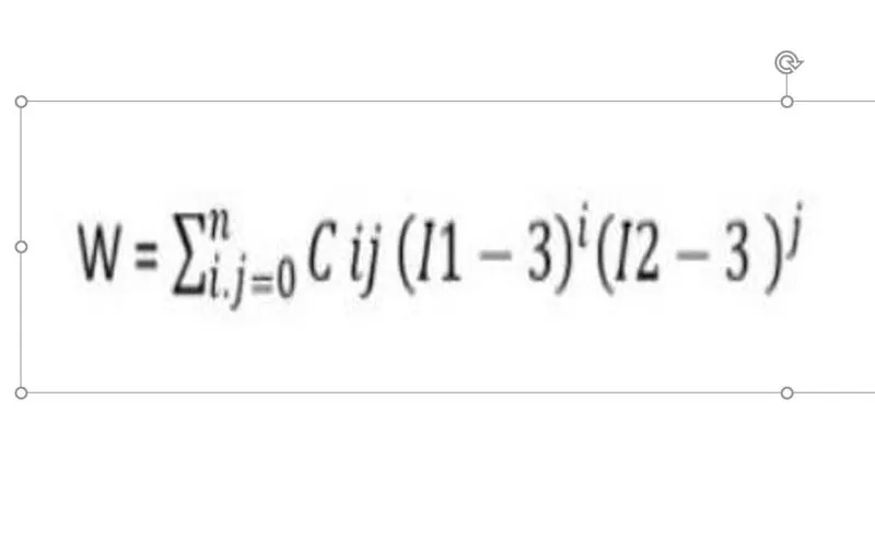
Where are empirically determined material constants, and are the first and the second invariant. By varying the Index values of and we can change the constitutive equations and use it appropriately for our component. Similarly, we will Cij I1 I2 i j be having multiple coefficients C. This changing of the index will be basically changing the order of the polynomial of the energy density equation.

We need to find out the coefficients of these material models for a different order of the polynomial and extract the best fit curve data from the D3HSp file and compare it with the material curve.

Procedure :-

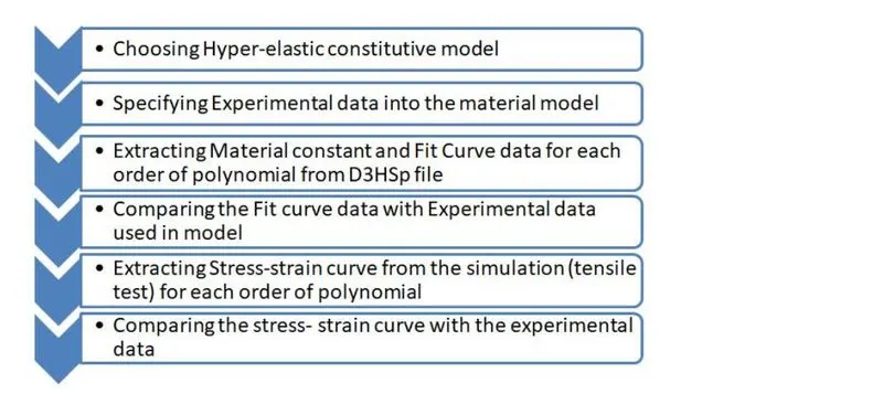
Workflow:

Hyper-elastic Material Card

As we are modeling a hyperelastic card, it is mandatory to use a material card that can access the necessary parameters pertaining to that of a hyperelastic material.

The following cards can be used to model a hyperelastic material,

1. *MAT_007 *MAT_BLATZ-KO_RUBBER- This is Material Type 7. This one parameter material allows the modeling of nearly incompressible continuum rubber. The Poisson’s ratio is fixed to 0.463.
2. *MAT_027 *MAT_MOONEY-RIVLIN_RUBBER-This is Material Type 27. A two-parametric material model for rubber can be defined.
3. *MAT_077_h *MAT_HYPERELASTIC_RUBBER This is Material Type 77. This material model provides a general hyperelastic rubber model combined optionally with linear viscoelasticity
4. *MAT_077_o *MAT_OGDEN_RUBBER This is also Material Type 77. This material model provides the Ogden rubber model combined optionally with linear viscoelasticity

Apart from these common hyperplastic materials for rubber there other material models too such as MAT_031, 038, 057, 063, 083, 092, 127, 129.

However, MAT_007 is a very simple rubber model with just one parameter to defined i.e. (Shear Modulus) we cant be used for our case and MAT_027 represents Mooney Rivlin constitutive model but this MAT_27 will only solve with First order of polynomial

So we will use MAT_077_h which represents Mooney Rivlin constitutive model and Different order of polynomial from 1 to 3 and find the Material constant for each order we can import a Load curve (experimental data value) and set SGL, SW, and ST parameters as 1 if the load curve is stress vs strain data.

Defining The Experimental data in the Material model

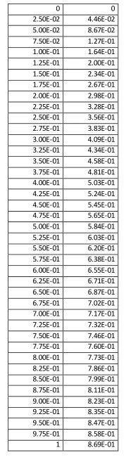
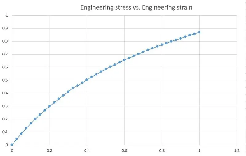
The stress/strain for the material is now in the form of Engineering stress and Engineering strain which can be directly implemented on the MAT_77h material card without any conversion

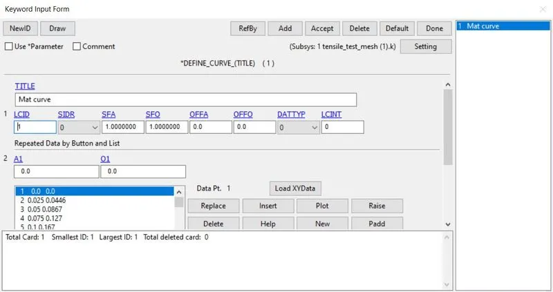
These data point for the Stress/Strain curve are inserted *DEFINE_CURVE Card with LCID

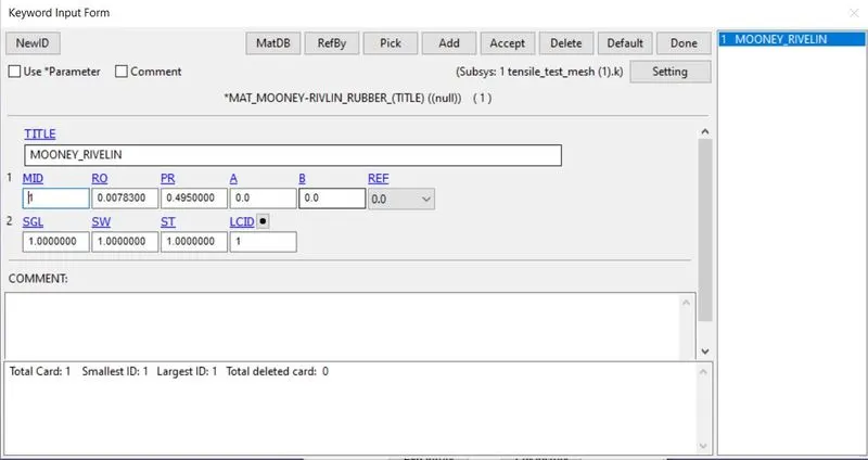
Material Card

1. MID Material identification. A unique number or label not exceeding 8 Characters must be specified
2. RO Mass density= 0.00100
3. PR Poisson’s ratio = 0.49100
4. N Number of constants to solve for = 1-3 for each case
5. LCSS Load curve ID defining Engineering stress versus Engineering strain LCID from *DEFINE_CURVE

Tensile Test – Pre Processing

Procedure:

• Mesh model of Dog bone specimen is imported
• The material model we created for graphite iron casting is used here
• Section shell card is used with 16: Fully integrated shell element formulation and thickness as 1mm

Boundary Condition

Since we performing a Tensile Test where one end of the specimen is fixed and the displacement is added to the other end so we will use two types of boundary condition on the Specimen

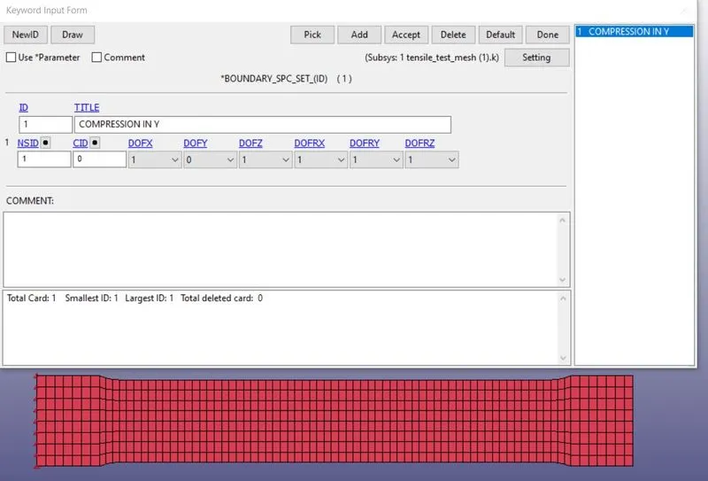
1. BOUNDARY_SPC_SET

• To fix one end of the specimen as test procedure we will constraint all the degree of freedom expects Y direction (because specimen will elongate in the X direction and simultaneously contract in Y) for edge node on one end of the specimen

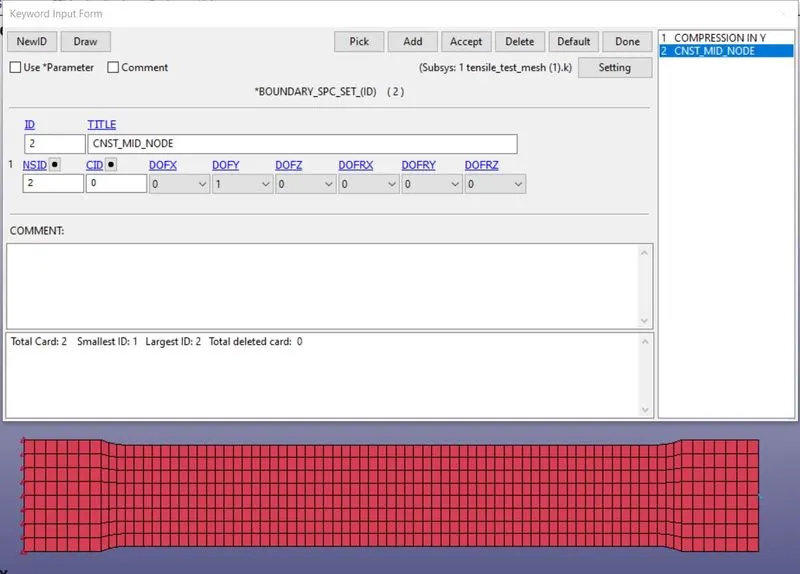
• We will select the mid-node on edge of both ends of the specimen and constrain only the Y direction

2. BOUNDARY_PRESCRIBED_MOTION_SET A set of a node is created on the edge specimen in which displacement is applied In the tensile test, the strain value as to be 100%. So we need to have the displacement same as the length of the specimen. The specimen length is 145 mm. So we need to have the displacement also as the 145mm.

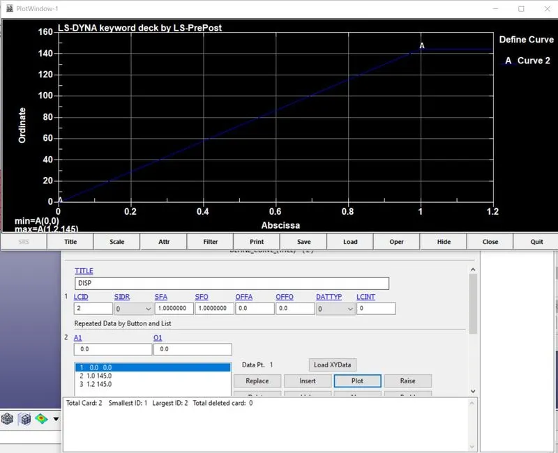
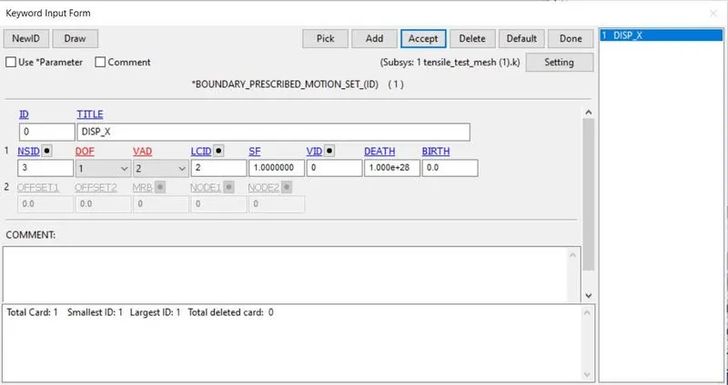
DOF in BOUNDARY_PRESCRIBED_MOTION_SET is set to be 1 which means displacement takes place in the X direction and VAD is set as 2 Displacement flag

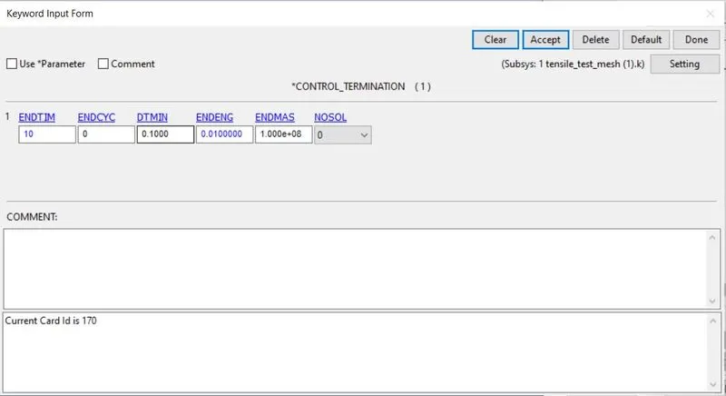
Control card

The termination time is set to 10ms

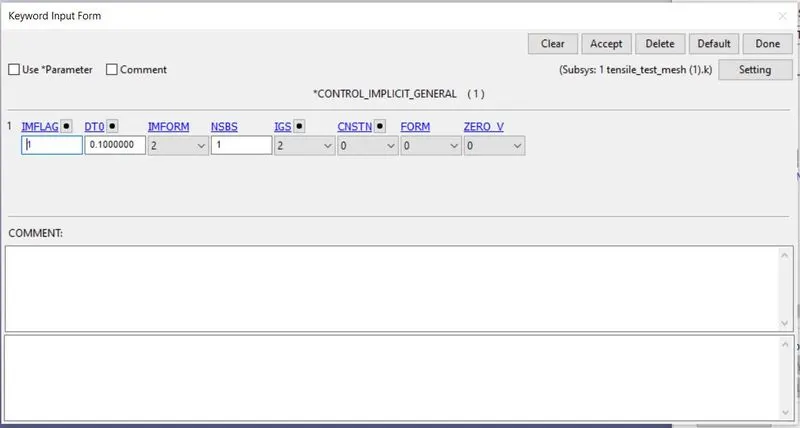
CONTROL_IMPLICIT_GENERAL

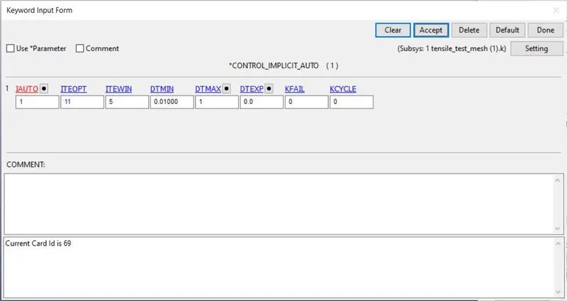
CONTROL _IMPLICIT_AUTO

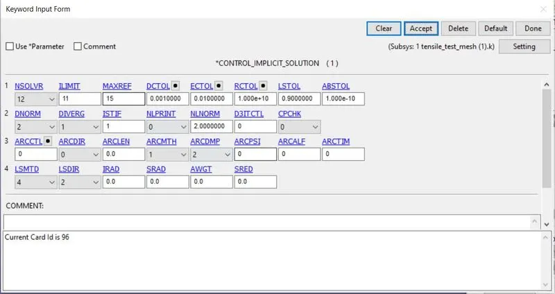
CONTOL_IMPICIT_SOLUTION

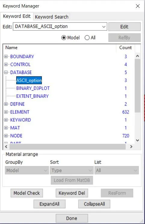
Database option :-

Running the Simulation (Mooney-Rivlin):

Now we will run the simulation.

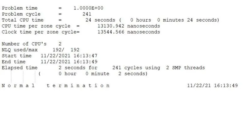
As we can see the simulation has a run-time of 24 seconds.

Comparison with input data :

We can obtain the stress/strain data after the initialization of the simulation from the d3hsp file.

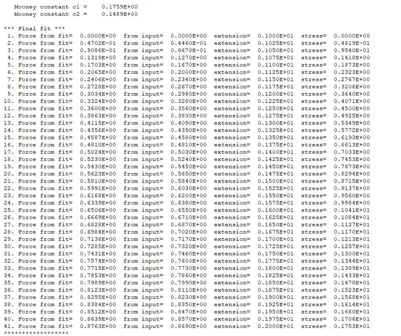
The constants c1 & c2 are noted down. We take the extension/stress data from this file and copy it to an excel sheet. To obtain strain from extension we subtract it by 1.

Also the stress value obtained here is true stress, we need to convert it to engineering stress to compare it with our input data.

We have the formula : Engineering stress = True stress/(1 + engineering strain)

Hence we obtain the engineering stress/strain values from this data.

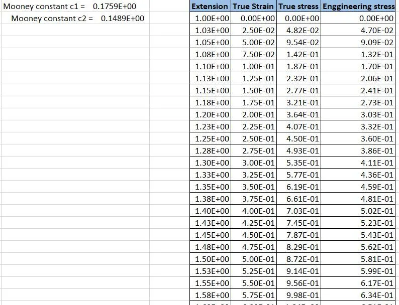
We then plot the data obtained from the simulation alongside the input data in a graph format like this to validate the results.

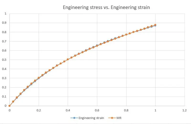
Hence we can see the data from the simulation matches correctly with our input data.

Comparison with constants input simulation :

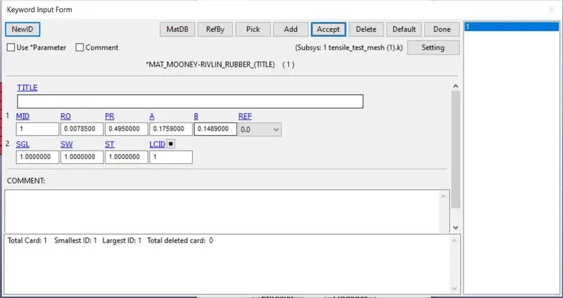
In the above simulation we entered the material data using a load-curve. Now we will enter the material data using the constants that were generated during the simulation run and see if we get a matching result.

Creating material card :

Mooney constant c1 = 0.1759E+00

Mooney constant c2 = 0.1489E+00

We will enter the above 2 values in the A& B column option instead of inputting the load curve as shown below.

Run the simulation :

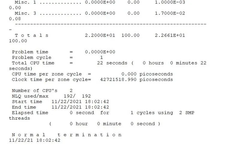
We see that the simulation now runs 2 second quicker and completes by 22 seconds as shown above. To compare the result the stress -strain curves are plotted for the element number 295 in both the cases. This element lies in the middle of the dog-bone specimen and will help us get a good result.

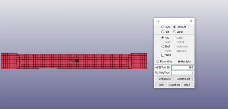
The stress -strain curve values are copied to an excel sheet and a graph is plotted as shown below.

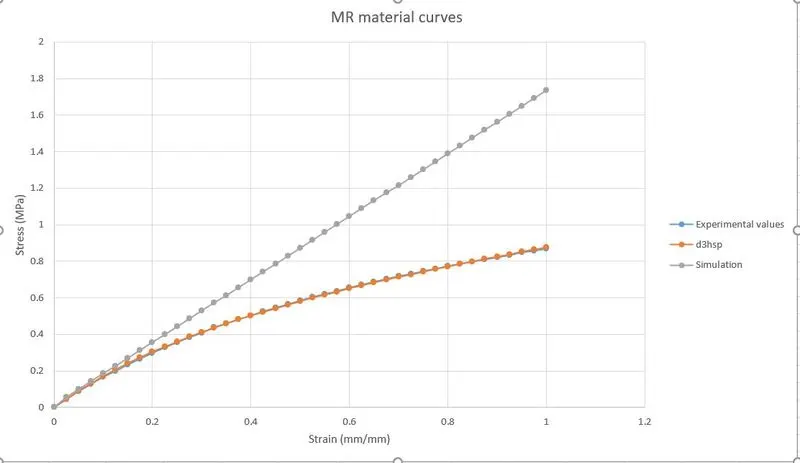
As we can see the results is not identical as the curve are not matching with one another. Because simulation curve is depending upon the material properties like poisons ratio and density since we approximately defined the values so we can’t expect to match curve properly.

Ogden material card

Creation of Material Card (Ogden) :

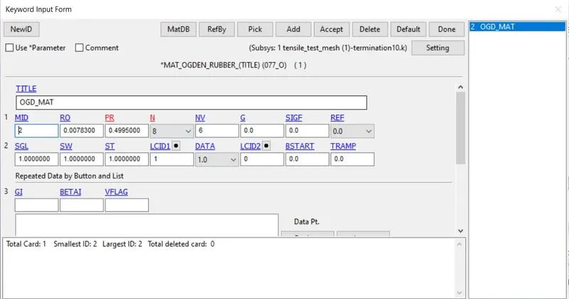
To create the Ogden material card create type 77 card as shown below, enter density, Poisson's ratio and N=8 to generate maximum number of constants so we can validate it better.

Enter SGL, SW, ST as 1 and enter the load curve. In Ogden material card we must define the strain for a greater value than what is supposed to run in the simulation. Hence to get a strain of 1 we must define the stress strain curve for a strain value more than 1.

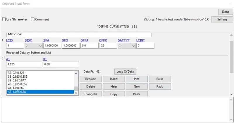
We will insert an additional point for strain of more than 1looking at the previous point and provide an arbitrary stress value as shown above. The rest of the simulation is exactly the same. So we will run it.

Running the Simulation (Ogden):

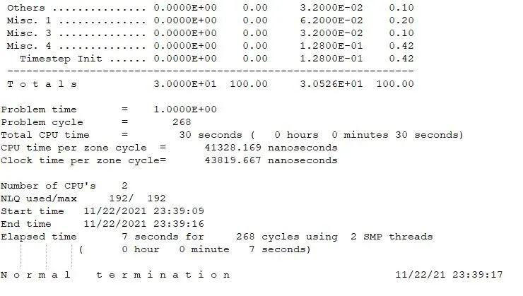
The simulation has a run-time of 30 seconds as shown above.

Comparison with input data:

We can obtain the stress/strain data after the initialization of the simulation from the d3hsp file.

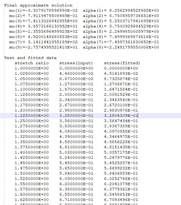
The constants

mu1, alpha1

mu2, alpha2

mu3, alpha3

mu4, alpha4,

mu5, alpha5,

mu6, alpha6,

mu7, alpha7,

mu8, alpha8

are noted down. We take the extension/stress data from this file and copy it to an excel sheet. To obtain strain from stretch ration we subtract it by 1.

The stress value obtained here is Engineering stress, so there is no need to convert it and we can directly compare it with the input data.

Hence we obtain the engineering stress/strain values from this data.

We then plot the data obtained from the simulation alongside the input data in a graph format like this to validate the results.

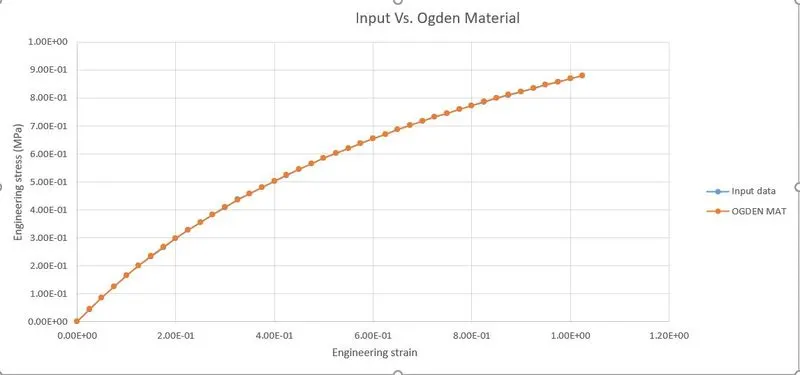
As we can see the data is more accurate and matches the input data more accurately when compared to MooneyRivlin material. Upto 2 decimal places the values match the input data exactly.

Comparison with constants input simulation:

In the above simulation we entered the material data using a load-curve. Now we will enter the material data using the constants that were generated during the simulation run and see if we get a matching result.

Creating material card :

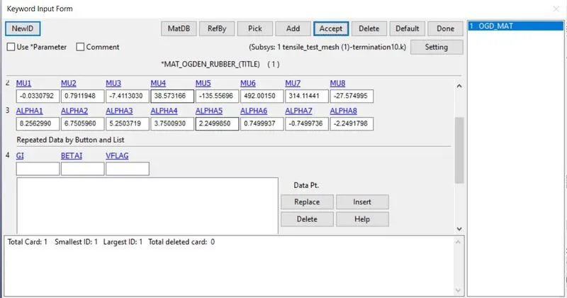
mu(1)=-3.3079178896590E-02 alpha(1)= 8.2562994528985E+00

mu(2)= 7.9119479508469E-01 alpha(2)= 6.7505959736651E+00

mu(3)=-7.4113028842955E+00 alpha(3)= 5.2503717941695E+00

mu(4)= 3.8573166130952E+01 alpha(4)= 3.7500929884529E+00

mu(5)=-1.3555696499923E+02 alpha(5)= 2.2499850005979E+00

mu(6)= 4.9200148680653E+02 alpha(6)= 7.4999369873616E-01

mu(7)= 3.1411441855189E+02 alpha(7)=-7.4997361830650E-01

mu(8)=-2.7574995521410E+01 alpha(8)=-2.2491799550008E+00

We will enter the above 8 values in the mu and alpha columns instead of inputting the load curve as shown below. Keep N= 0 to get constants input mode in the material card.

Run the simulation:

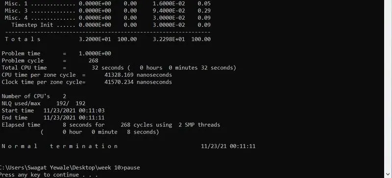
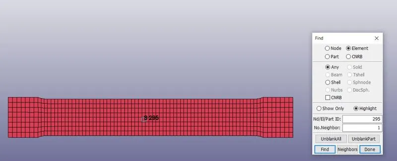
To compare the result the stress -strain curves are plotted for the element number 295 in both the cases. This element lies in the middle of the dog-bone specimen and will help us get a good result.

The stress -strain curve values are copied to an excel sheet and a graph is plotted as shown below.

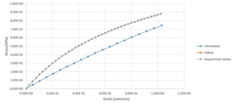
As we can see the results is not identical as the curve are not matching with one another. Because simulation curve is depending upon the material properties like poisons ratio and density since we approximately defined the values so we can’t expect to match curve properly.

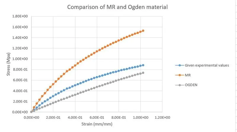
Comparison of 2 Material curves:

We will compare the input data to the data obtained by the fit from both the material cards to obtain the following graph below. As we can see Ogden model is more accurate than MR material.

Conclusion:

Hence we have studied both the material cards to validate that the simulation is performing exactly like the test input data. We arrive at 2 conclusions:

1. The Ogden material model is slightly more accurate than Mooney-Rivlin material card but is computationally more expensive.
2. Hyper-elastic material cards can be defined using Constants or Load Curves to get identical results. However, entering constants proves to be computationally less expensive.