Week - 9 Material Modeling from Raw Data

Material Modeling from Raw Data

AIM: To create a material model using the data extracted from the given true stress-strain curve of graphite iron casting and validate it using the dog bone specimen.

Problem statement :-

Use the diagram of the true stress-strain curve of graphite iron casting. Two curves are there for different material structures. Students need to pick any one of them and use the data to create either a MAT_024 or MAT_018 material model and then validate it.

Here is the workflow:

1. Extract the data from the diagram
2. Clean the data and visually confirm that it matches the original data and the elastic modulus is 20.9E+06 psi.
3. Convert the data to (kg-mm-ms) unit system
4. Process the data and create the material as demonstrated
5. Use the material model with a dog-bone specimen and validate the same.

INTRODUCTION:
Material model: To get realistic results for any analysis using FEA, a good material model for the material is necessary. A material model can have all sorts of data describing the behaviour of the material in different conditions: say different tensile test curves for different strain rates and much more. This helps getting realistic behaviour of the component with the material model in all sorts of situations.

Building a material model requires test data from various experiments conducted in real life to describe the material behaviour in detail. A complex analysis would benefit from a detailed material model, whereas a simpler simulation would not benefit much. The data collected from an experimental test is first cleaned to make sure any unnecessary data points are filtered out to get clear picture. Usually, the same test is repeated a number of times to ensure repeatability of the results. This test data is then inserted in the suitable format into a model: say effective stress-strain curve in x-y coordinates.

A cleaner data with consistence behaviour in the case of a stress strain plot, inconsistent data points should be avoided as it can affect the stability if the simulation having such a material model. A fitted curve with 98%+ accuracy can solve such issues. After matching for the unit system of the analysis, this data can be added to the simple material model to make it more detailed – for example with the use of material model such as MAT24 – linear piecewise material.

A good practice of the material modelling procedure is the validation of the model. By performing simple analysis for which an experimental test can be performed or such data can be acquired, and then comparing the experimental and analysis results gives a good benchmark for the model. In this exercise, we try and replicate such a process.

Material modelling is done with the help of raw data. We have to extract the data from given image. The given image gives you the Engineering Stress and Engineering Strain values. These values will produce the True stress and true strain with the help of calculations.

PROCEDURE:

1.Data Extraction: The given image file of true stress-strain graph of graphite iron casting is opened in data digitizer software to extract the data and export it as excel file.

The curve 2 is chosen to extract data of stress-strain of graphite iron casting as shown in fig.1.

Note: Ensure the data points picked is evenly spaced so as to get smooth curve and better convergence.

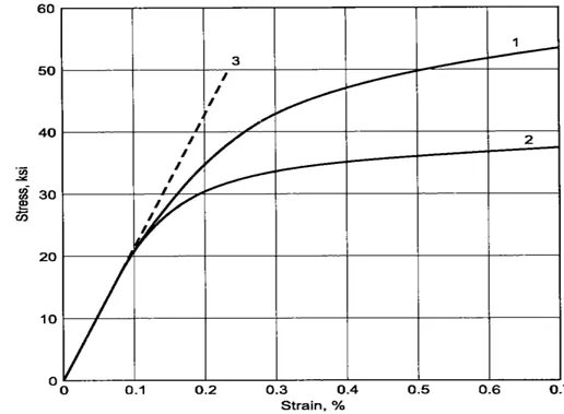
Fig. Given image and points for data extractions.

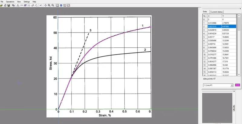
Fig.2 Plot of true stress vs true strain of curve 2.

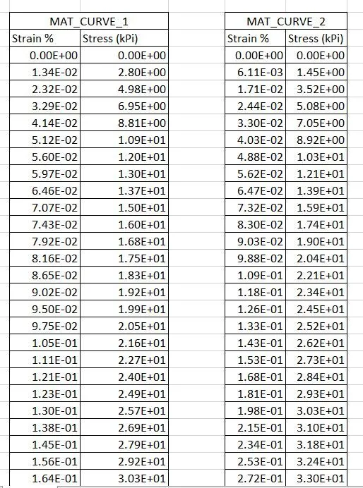
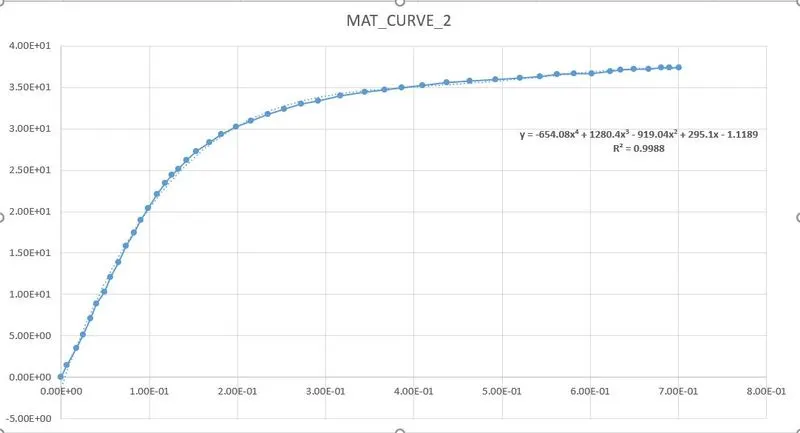
2. The stress-strain data file obtained from data digitizer is opened in excel to plot a graph of true stress, (GPa) vs true strain as shown in fig. From the graph the yield stress value is taken as 21.90 ksi which is 0.151 GPa and the region beyond is considered as plastic region.

3.The true stress-strain data is then converted into effective plastic strain and stress to add to the material card. To keep the plot consistence, a curve is fitted to the extracted data, and the data-points are taken from the curve. Using the following relation, the true stress-strain data is converted into effective plastic stress-strain data:

True strain = ln (1+ Engg, strain)

Effective strain = Total true strain - (true stress/Young's modulus)

True Stress = (engineering stress) * exp(true strain)

= (engineering stress) * (1+ engineering strain)

for metals, 'E' is large (100 x GPa), hence (true stress/E) can be taken as constant for all the points in the test data. This DOESN'T hold true for plastics where E is comparatively low (1x GPa).

4. The acquired data is input as a curve, and then recalled in the material model- MAT24. 4. A tensile test model is setup for the given dog-bone model, where the boundary conditions are:

• One end is fixed with all DOFs locked except translation in lateral direction to allow the compression.
• All nodes on the other end are added to a node_set to which a ‘prescribed_boundary_condition’ of displacement is applied in the longitudinal axis.
• The middle node on each of the ends is constrained in all other DOF except translation in the longitudinal axis to avoid contradicting boundary conditions and keep the loading tensile in nature.
• A linear displacement curve is defined to get cover good part of the experimental test with as much plastic straining as possible without getting into instabilities.
• The necessary outputs were requested in ‘database’ keyword and the results were compared to the input curves.
• To understand the process better an implicit analysis is performed for the same to observe the stress distribution, and overall results.

5. From the plot it can be observed that there are some inconsistencies in the plot hence a curve is fitted to it using trendline feature in excel. It is made sure that the error is minimal. Given the nature of the graph, a logarithmic distribution gets a very close fit and hence is selected. To match a suitable unit system, the units for stress were converted from KSI – Kilo pounds per square inch into GPa – Giga Pascal using following conversions:

1 Kilo Pounds per square inch = 4.44822 KN = 6.8947572 Pascal.

To get good results we have make some equidistant spacing in the strain % so it will produce the curve which will result monotonically increasing values

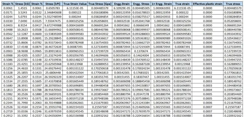
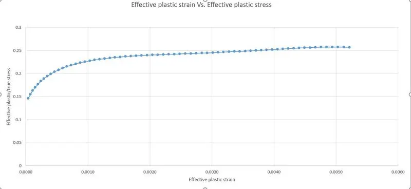
Fig.4 Plot of effective stress vs effective strain

Analysis Model and setup:

The given dog-bone specimen keyword file only has the mesh data and hence everything else needs to be added. To keep the analysis simple yet informative, the before mentioned boundary conditions were added along with a MAT24 material the analysis simple yet informative, the before mentioned boundary conditions were added along with a MAT24 material model consisting of the ‘log-data’ acquired from the experimental results. After trying a number of times to get the required results without any instability and unusual results, the following settings were finalized.

Part Definition: 1. The material card chosen is MAT_24_PIECEWISE_LINEAR_PLASTICITY to define the behavior of an elasto-plastic material with an arbitrary stress versus strain curve and arbitrary strain rate dependency. With this material model it is possible to consider the effect of the strain rate.

• The values of density and Poisson’s ratio is taken as generic values.
• The given value of young’s modulus = 20.9E+06 psi = 144.1004 GPa.
• The yield stress value from the graph = 0.151 GPa.

2. The curve LCID1 is defined using *DEFINE_CURVE engineering stress versus engineering strain.

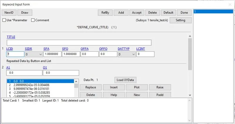
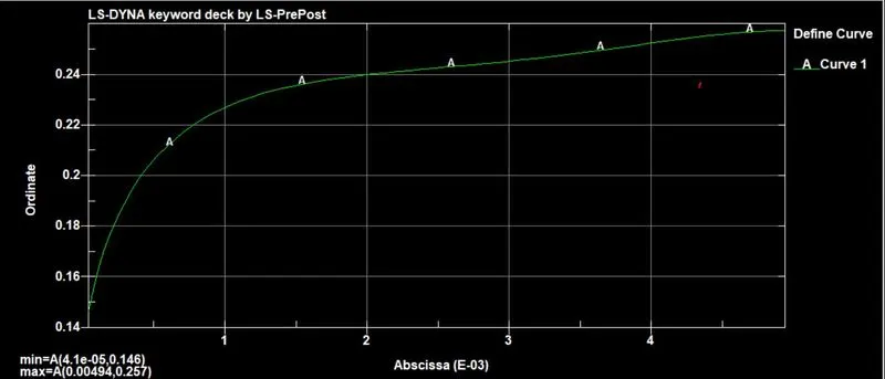
Fig. Defining curve - A

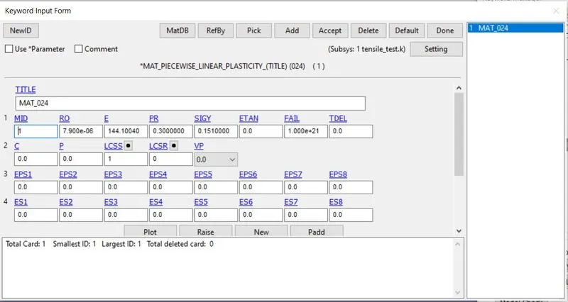
Fig. LCSS curve definition for EPS vs ES

The plastic behavior of the material is defined using LCSS curve option in the material card. The curve is defined by inputting the values of effective plastic strain and effective stress (true stress).

The Effective Plastic Strain = True Strain – (True Stress/Young’s Modulus).

Note: To define LCSS curve the stress values beyond the yield stress values are considered.

SECTION PROPERTY

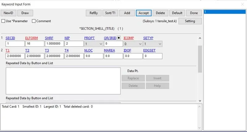
The section property of dogbone specimen is assigned as shell element with 2 mm thickness and ELFORM=16.

PART DEFINATION

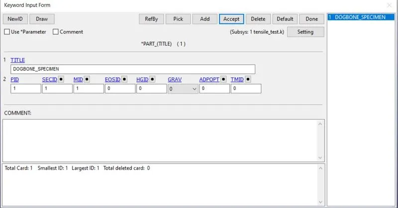
3. Boundary Condition: The nodes at the fixed end are constrained in X and Z direction only and Y direction is not constrained because of lateral expansion during tensile test

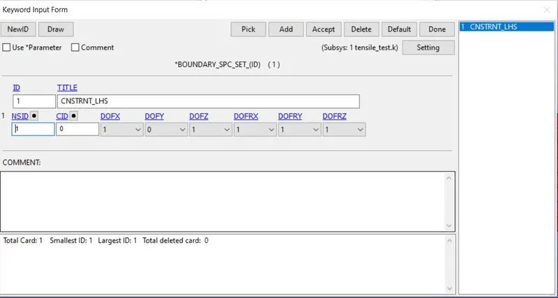
Fig. The nodes at the fixed end constrained in X and Z direction.

The nodes at the fixed end is constrained in X and Z direction only and Y direction is not constrained because of lateral expansion during tensile test.

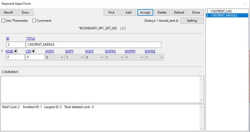
Fig. The nodes at the middle constrained in Y direction.

The nodes at the middle are constrained in Y direction since the neutral axis passes through the middle of the specimen in Xdirection.

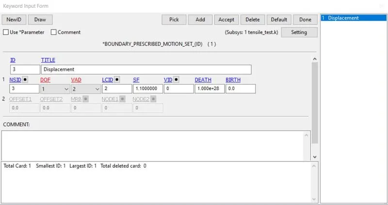
Fig. Boundary prescribed motion in the pulling end of specimen.

The nodes of the pulling end are assigned with a boundary prescribed motion in X direction using displacement load curve as shown in fig.

Database Options: The time step value for the BINARY_D3PLOT and DATABASE_ASCII option for GLSAT and ELOUT is given as 0.01 ms. DATABASE_EXTENT_BINARY card with STRFLG =1, is used to compute the elastic strain in the model.

Control Functions: The tensile test of given dog bone specimen is considered as quasi-static analysis, hence implicit analysis is carried out with necessary control implicit cards as shown in fig.10. The Initial time step size for implicit analysis, dt0 =0.025.

Note: The value of dt0 should be chosen wisely for better convergence.

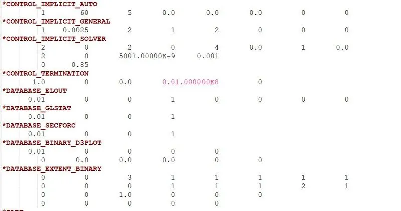
Fig. Control functions for implicit analysis.

RESULTS AND DISCUSSIONS:

1. The animation of Von-Mises stress contour.

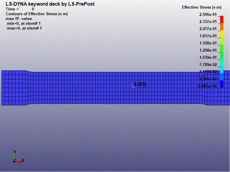
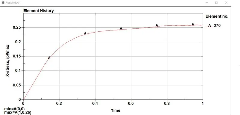
The animation of stress and strain contour resemble realistic simulation of tensile test. The maximum v­m stress value is 0.2596 GPa which is higher than the yield stress value of 0.151 GPa. Hence, plastic deformation is occurring in the specimen. The maximum stress is developed in the middle region of specimen but necking is not observed till the end of simulation.

2. The animation of Effective Plastic Strain contour.

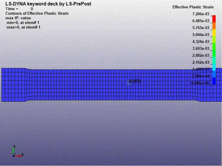
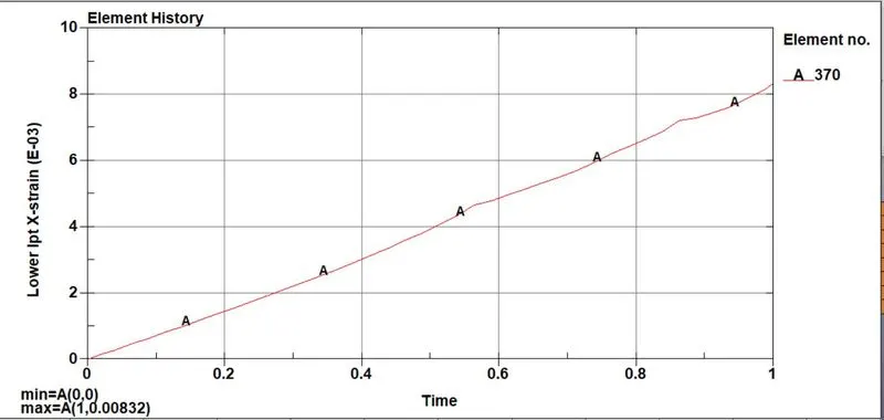
The maximum effective plastic strain observed is very less as 0.007206 Due to plastic strain the cross section of specimen is decreasing at the middle of specimen.

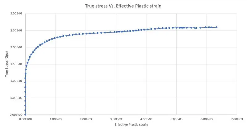
The true stress vs true strain plot obtained from simulation of tensile test on dog bone specimen is as shown in fig. which resembles the given true stress vs true strain plot.

3. True stress vs. effective strain

4. Result validation

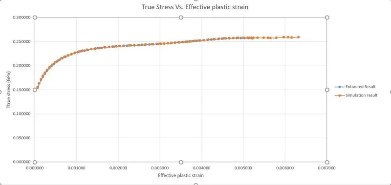
Fig. Validation of simulation results with raw data.

From the graph, the curve of raw true stress vs true strain plot exactly fits with simulation result curve of true stress vs true strain plot with dt0 = 0.0025.

CONCLUSION:

1. The stress-strain data was extracted from the given diagram using data digitizer.
2. The extracted stress-strain data is used to model material using MAT_24 material card.
3. The material model is validated using tensile test on dog bone specimen by implicit analysis.
4. Learned to model material from raw data and validated it.