Assignment 3-2D Element Formulation Challenge

Crash Beam simulation using Radioss

Aim :- To simulate the crash beam with default element properties and with a given elements property and compare their results with plot of forces and various energies.

Software used :- Altair hyper-works student version 2020

Problem statement :-

Comparison of results with base simulation and improved shell element properties

1.Using the crash beam file from the previous assignment, change the run time to 55 ms.

2. Change the number of animation steps during simulation to a minimum of 25 and maximum of 60.
3. Run the base simulation without any modification to element properties.
4. At the end of the simulation, do the energy error and mass error checks and determine whether results would be acceptable.
5. If acceptable, Plot rigid wall forces, internal energy, hourglass energy, contact energy, total energy of the simulations.
6. Change all the shell elements properties to recommended properties, save this as separate, rad files and run the simulation.
7. Follow steps 5 and 6.
8. Create a brief report comparing all the results from steps 5 and 6 for both simulations.
9. Comment whether there is any change in the results and why there is any change in the result.

Recommended properties:

Parameters	Comment
Ishell =24	QEPH 4 nodes shells are best combination of cost and accuracy.
Ismstr=2	Full geometric nonlinearities (default)with possible small strain formulation activation in RADIOSS Engine.
Ish3n=2	Standard 3 noded shell (C0)with modification for large rotation(default)
N=5	Number of integration points set to 5 for accuracy bending.
Ithick=1	Thickness change is taken into account for accuracy.
Iplas=1	Iterative plasticity for good accuracy.

Solution :-

Case 1 :- Without changing the properties of element.

1. Opening given .rad file

Import given model into hyperworks , given model is not .hm format so use import solver deck in toolbar > select starter file which stored in _0000.rad format > Import option as shown in image below.

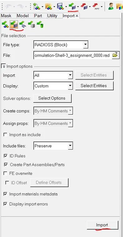
Fig. 1 Importing starting input file

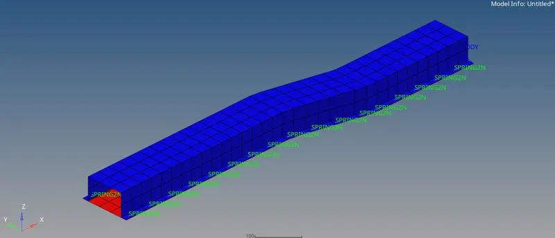
Fig.2 Given model

2. Changing run time as per problem statement. :-

As per problem statement we need to change the run time to 55 ms. for that, select cards > ENG_RUN menu > Change the T_stop value to 55ms option. It will change the run time of simulation.

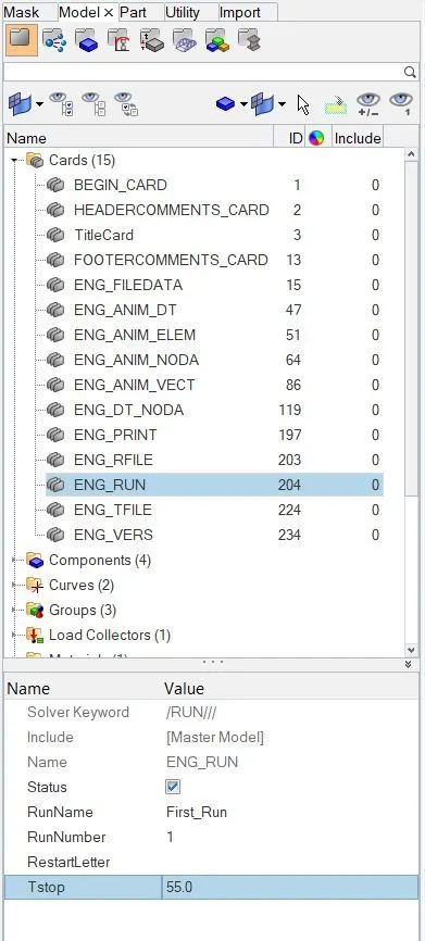
Fig.3 Setting Tstop

3. Change the number of animation steps during simulation to a minimum of 25 and maximum of 60 :-

Frequency = Termination end time / Steps required

= 55/50

T_freq = 1.1

Set T_freq to 1.1 In ENG_ANIM_DT cards as shown in image below.

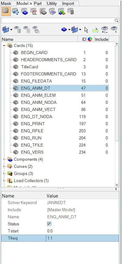
Fig. 4 Engine animation card

4. Run the simulation with default properties :-

For running simulation go to following path Analysis > Radioss > select path where model need to be saved > select export option as a all > run option as a analysis > run number as a1 > type -nt 4 in options for increasing simulation speed > Radioss. It will take few seconds time for calculating simulation. It will pop-up Radioss job complete window as shown in image below.

Fig. 5 Analysis > Radioss deck

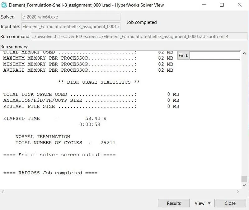
Fig.6 Radioss job complete window

5. Switch the client selector to Hyperview from hypermesh, and open .h3d file and click on apply. The simulation will start as a press the start animation button.

Fig 7. Loading of .h3d file in hyperview

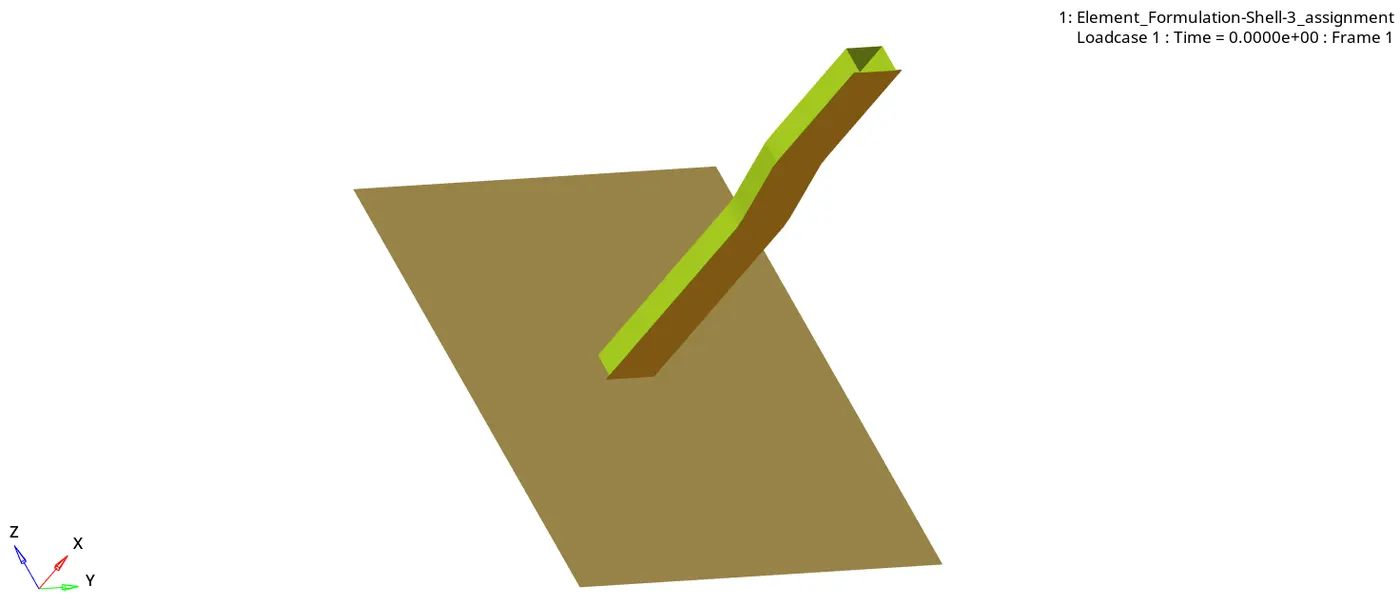
Fig 8 Simulation in first Case

6. Open output file and check energy error and mass error as shown in image below.

Fig. 9 Energy error and mass error from output file for first case

From output file energy error is -10.3% which is negative and decreasing step by step since the energy error should be -15% to -5% for accepting results so we can accept the results and plot the graphs.

7. Split the screen into two windows and extend second window and switch client view as a hyper graphs 2D and select X type – Time > Y type – Global variables > Select Internal energy, Kinetic energy, Hourglass energy and total energy > Select magnitude > Preview it will shows the graph for Selected Energies with respect to time as shown in image below.

Fig. 10 Selection of graph parameters

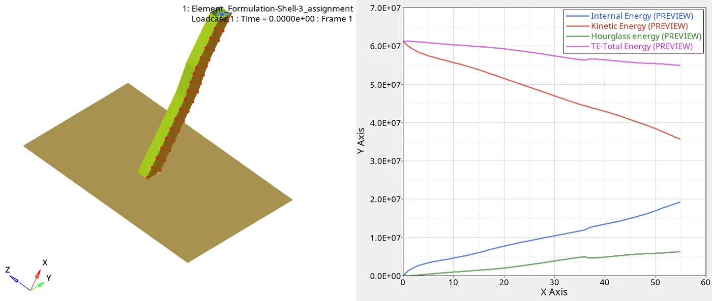
Fig. 11 Energy graph for default properties

7. Similarly, open new window and in hyper graph 2d plot the graph for rigid wall forces which is shown in image below.

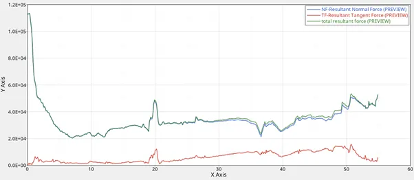
Fig. 12 Forces acting on rigid wall graph for default properties

Case 2 :- With changing recommended properties of element.

1. For case 2 assign recommended properties to components for shell element formulation as shown in image below.

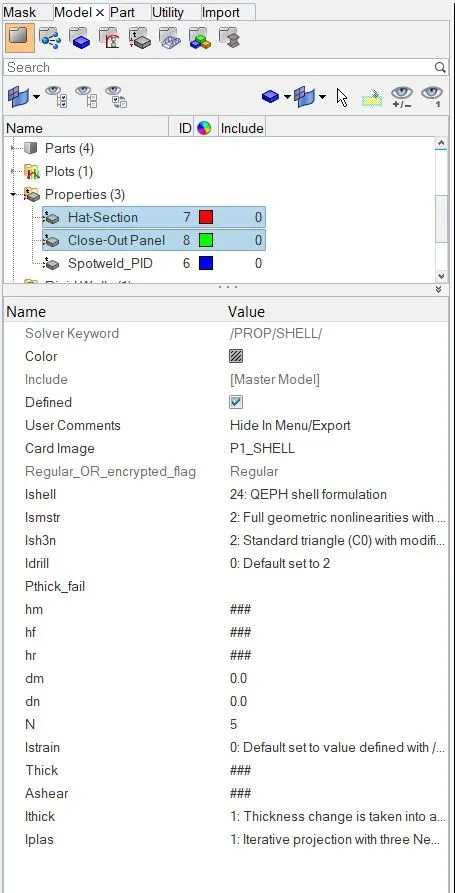
Fig. 2.1 Assigning recommended properties

2. For simulation same procedure is to be followed on case 2 model as we done on case 1.
3. Click on the result tab to view animated file of simulation of model as shown in image below.

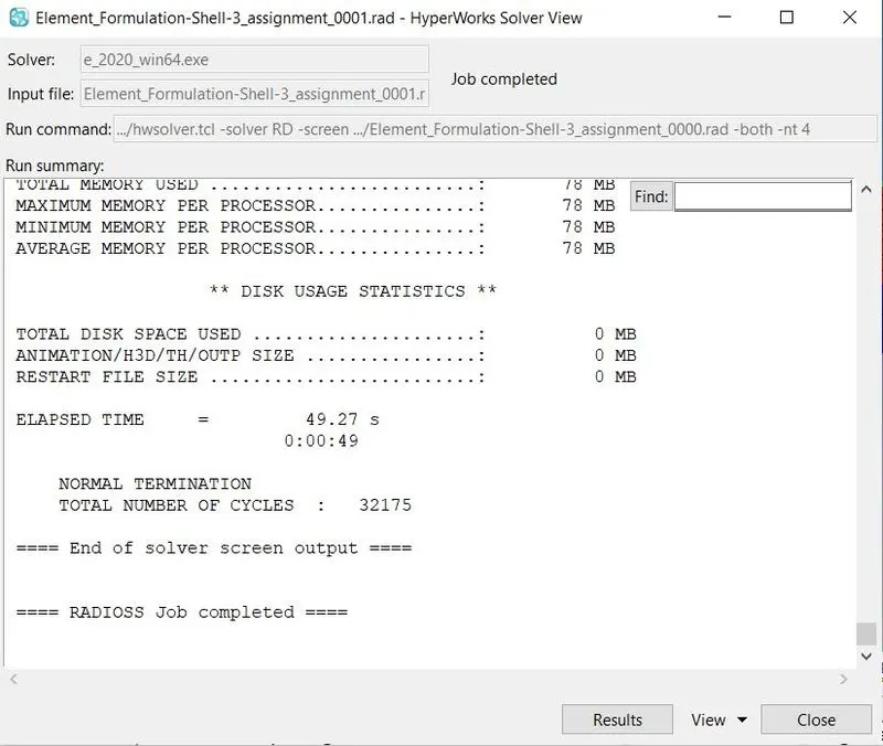
Fig.2.2 Radioss job complete window

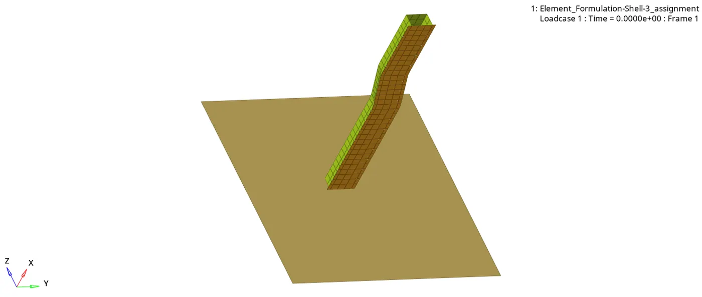
Fig 2.3 Simulation in Case 2

4. Open output file and check energy error and mass error as shown in image below.

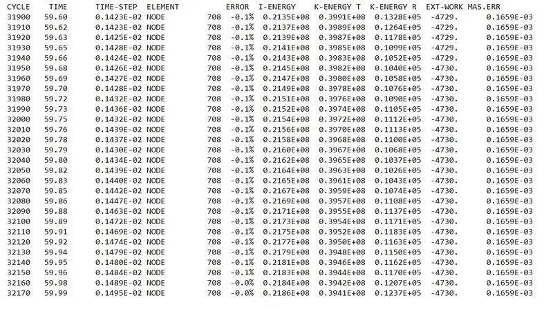
Fig. 2.4 Energy error and mass error from output file

From output file energy error is -0.1 % due to no hourglass energy formulation. Since for QEPH shell formulation the energy error should be 1% to 2% for accepting results so we can accept the results and plot the graphs.

5. Split the screen into two windows and extend second window and switch client view as a hyper graphs 2D and select X type – Time > Y type – Global variables > Select Internal energy, Kinetic energy, Hourglass energy and total energy > Select magnitude > Preview it will shows the graph for Selected Energies with respect to time as shown in image below.

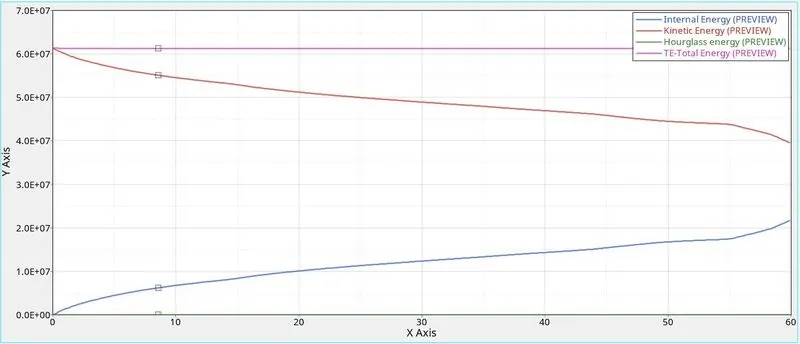
Fig. 2.5 Graph of energies with recommended properties

6. Similarly, open new window and in hyper graph 2d plot the graph for rigid wall forces which is shown in image below.

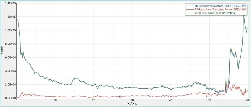
Fig. 2.6 Graph of forces acting on rigid wall

Comparison between Case1 and Case 2 :-

Fig. 12 Forces acting on rigid wall graph for default properties Fig. 2.6 Graph of forces acting on rigid wall

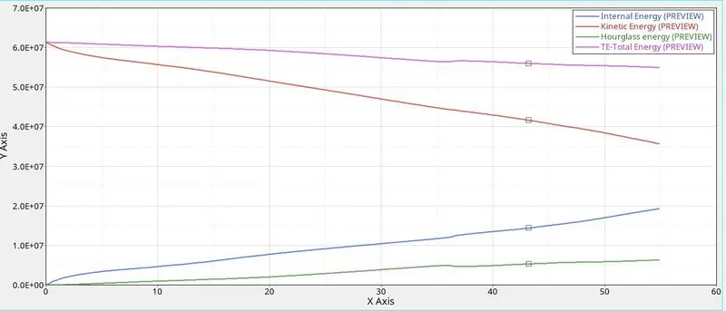
Fig. 11 Energy graph for default properties Fig. 2.5 with recommended properties

Fig. 2.4 Energy error and mass error from output file Fig. 9 Energy error and mass error from output file for first case

1. Internal energy generated with default property is 1.9E+07 J is less than the internal energy generated with recommended property which is 2.18E+07 J
2. Also there is small difference in kinetic energy at t=0
3. Hourglass energy is zero in QEPH shell formation elements ( Case 2) while there is generation of hourglass energy in Q4 shell formation elements ( Case 1)
4. In case 1 total energy is decreases while in case 2 graph of total energy is constant which is 6.01E+07 J
5. all the above energy differences are arises due to in Q4 (Default property ) elements hourglass energy is generated while in QEPH elements ( Recommended property) gives accurate results while loading and unloading. In Q4 hourglass energy is generated due to only one point of integration which results into hourglass formation. This can be resolved by two method Perturbation method and Viscous method.
6. In Q4 shell element formation energy error is -10.3% and mass error is 0.1659E-03 while in QEPH shell element formation energy error is -0.1 % and 0.1659E-03 which is very less than Q4 elements because it is fully integrated elements.

Conclusion :- Thus, the given model is simulated in both the Cases and acceptable results are obtained from both simulations. In QEPH case obtained results are more accurate in loading and unloading due to its higher number of integration points than Q4 elements also it is better option in terms of relative cost.