Week 7 - Simulation of a 1D Super-sonic nozzle flow simulation using Macormack Method
AIM:
To simulate the isentropic flow through a quasi 1D subsonic-supersonic nozzle by both the conservation and non-conservation forms of the governing equations using the MacCormack's technique.
OBJECTIVES OF THE PROJECT:
To show the following plots inside your report
1. Steady-state distribution of primitive variables inside the nozzle
2. Time-wise variation of the primitive variables
3. Variation of Mass flow rate distribution inside the nozzle at different time steps during the time-marching process
4. Comparison of Normalized mass flow rate distributions of both forms
THEORY:
Nozzle:
A nozzle is a device designed to control the direction or characteristics of a fluid flow (specially to increase velocity) as it exits (or enters) an enclosed chamber or pipe.
A nozzle is often a pipe or tube of varying cross sectional area, and it can be used to direct or modify the flow of a fluid (liquid or gas). Nozzles are frequently used to control the rate of flow, speed, direction, mass, shape, and/or the pressure of the stream that emerges from them. In a nozzle, the velocity of fluid increases at the expense of its pressure energy.
Converging diverging nozzle:
The usual configuration for a converging diverging (CD) nozzle is shown in the figure. Gas flows through the nozzle from a region of high pressure (usually referred to as the chamber) to one of low pressure (referred to as the ambient or tank). The chamber is usually big enough so that any flow velocities here are negligible. The pressure here is denoted by the symbol pc. Gas flows from the chamber into the converging portion of the nozzle, past the throat, through the diverging portion and then exhausts into the ambient as a jet. The pressure of the ambient is referred to as the 'back pressure' and given the symbol pb.
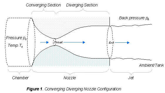
The nozzle converts the low velocity, high pressure, high-temperature gas in the combustion chamber into high-velocity gas of lower pressure and low temperature. Let a nozzle is used to get supersonic speed by the low speed at the inlet. The Mach number which gets an increase from inlet M=0 to M>0 at the outlet .nozzle always converges at the subsonic part and diverges at the supersonic part. This is pretty much clear that the Mach number is equal to unity (M=1) at the throat. Therefore sonic speed is always achieved at the throat. Fig 1 given below give a clear concept of it.
INTRODUCTION TO THE PHYSICAL PROBLEM: SUBSONIC-SUPERSONIC ISENTROPIC FLOW:
We consider the steady, isentropic flow through a convergent-divergent nozzle as sketched in Fig. The flow at the inlet to the nozzle comes from a reservoir where the pressure and temperature are denoted by p0 and To, respectively. The cross-sectional area of the reservoir is large ( theoretically, A is infinity), and hence the
velocity is very small ( V = 0). Thus, Po and T0 are the stagnation values or total pressure and total temperature, respectively. The flow expands isentrop1cally to supersonic speeds at the nozzle exit, where the exit pressure, temperature, velocity and Mach number are denoted by Pe, Te, Ve and Me, respectlvely. The flow is locally subsonic in the convergent section if the nozzle, some at the throat (minimum area), and supersonic at the divergent section. The sonic flow (M = 1) at the throat means that the local velocity at this location is equal to the local speed of sound. Using an asterisk to denote sonic flow values, we have at the throat V = V* = a*. Similarly, the sonic flow values of pressure and temperature are denoted by p* and T*, respectively. The area of the sonic throat is denoted by A*.
1. Governing equation:
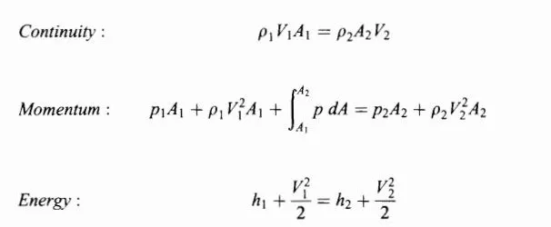
The governing continuity, momentum, and energy equations for this quasi-one-dimensional, steady, isentropic flow can be expressed, respectively, as
By solving, we get non-conservative form of governing equation as,
Non-conservative form:
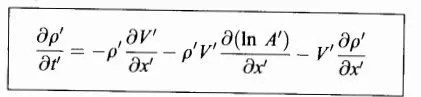
Continuity equation:
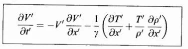
Momentum equation:
Energy equation:
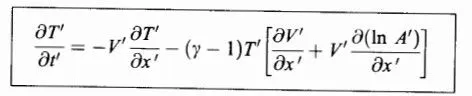
we get conservative form of governing equation as,
Continuity equation:
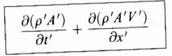
Momentum equation:
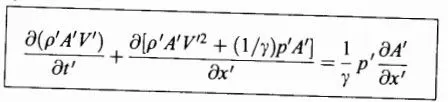
Energy equation:

2. Setting up of the finite-difference expressions using Mac-Cormack's explicit technique (non-conservative scheme)
Predictor step:
Continuity equation:

Momentum equation:

Energy equation:

Using the above values,we compute the predicted values of ρ,V,T as follows,
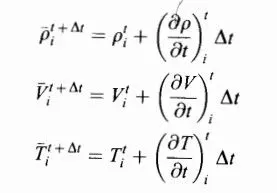
But these values are only 1st order accurate. Inorder to have 2nd order accurate, we need to da corrector step. In corrector step we proceed the same step as above in predictor step but with backward implicit scheme instead of forward implicit one.
3. Corrector step:
Continuity equation:
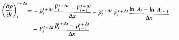
Momentum equation:

Energy equation:
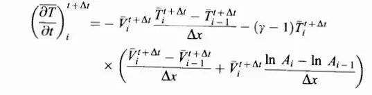
4. Computing average of predictor and corrector
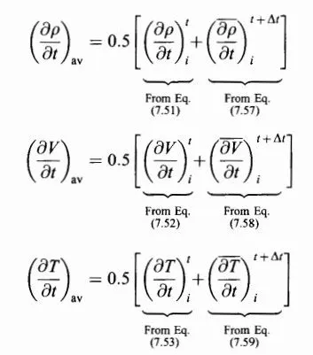
This will be the actual value in the next time step.Finally, we have for the corrected values of the flow-field variables at time t + ∂t
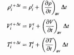
Calculation of time step:
Here, we need to know the value of 'dt' which is calculated by adaptive time step approach (minimum time step approach) where dt is given by formula as
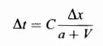
where C = CFL number which is generally less than or equal to 0.8, dx= grid spacing, a = velocity of sound which is non-dimensional value written as (T)^0.5 and 'V' is the velocity of the moving object.
So we get a series of 'dt' values since 'a' and 'V' are array matrix with 31 grid points. Now 'dt' is chosen from minimum time step approach.

5. Boundary conditions:
Next we apply boundary conditions which is obtained by taking slope of the adjacent two points of the initial and final point of the boundary and linear extrapolation is done.
Subsonic inflow.boundary (point 1)
We use linear extrapolation from points 2 and 3 to calculate Vi, This is illustrated equation below Here, the slope of the linear extrapolation line is determmed from points 2 and 3 as 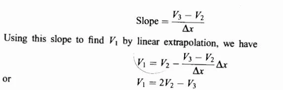
Supersonic outflow boundary (point N)
Here, we must allow all flow-field variables to float We again choose to use lmear extrapolation based on the flow field-values at the internal points, Specifically, we have, for the non-dimensional variables,
VN = 2VN-1 - VN-2
PN = 2PN-1 - PN-2
TN= 2TN-I - TN-2
Conservation form:
Basic Equations in Conservation Form:
Continuity equation:
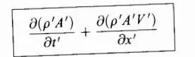
Momentum equation:
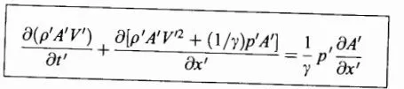
Energy equation:

Equations above are the non-dimensional conservation form of the continuity, momentum, and energy equations for quasi-one-dimensional flow, respectively. The equations for quasi-one dimensional flow can be expressed in a similar generic form. Let us define the elements of the solutions vector U, the flux vector F, and the source term J as follows. 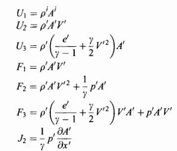
Thus the equation can be written as,
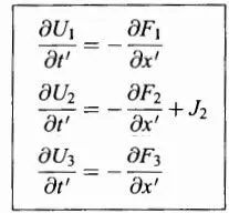
After solving and deriving the flux terms and residue terms in the form of solution vector we get,
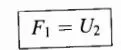
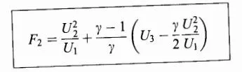
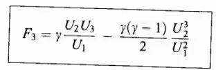
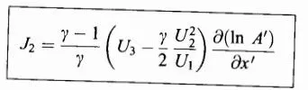
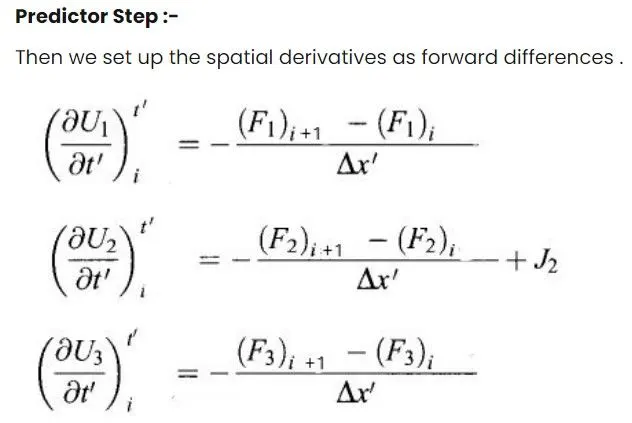
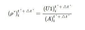
Finding U1,U2,U3 values from the predicted values
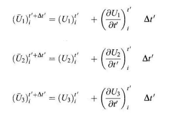
Corrector step:
The above step is repeated but with backward difference method.
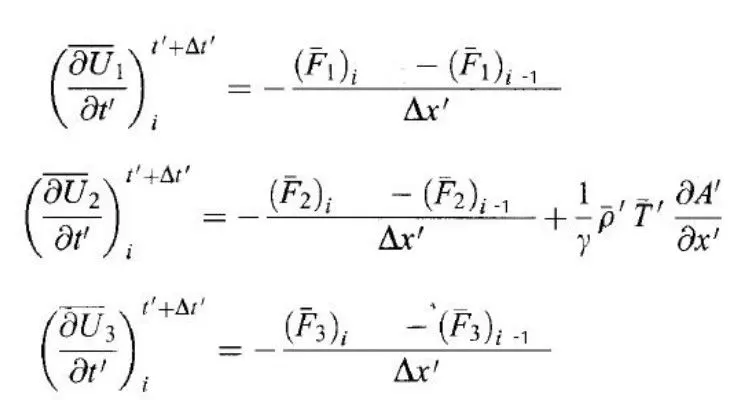
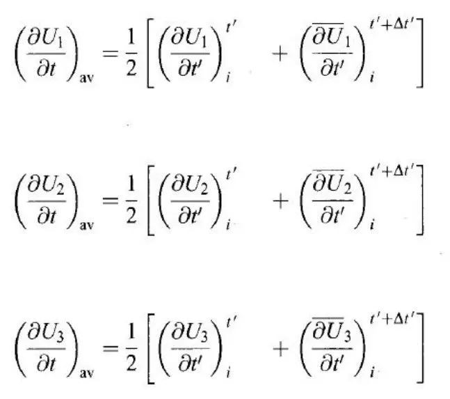
Computing average time derivatives,
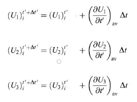
Computing final solution
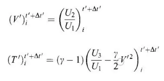
Computing primitive variables from the above computed values,
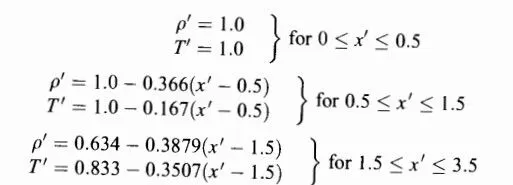
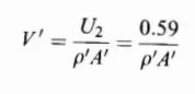
Initial conditions for conservative form:
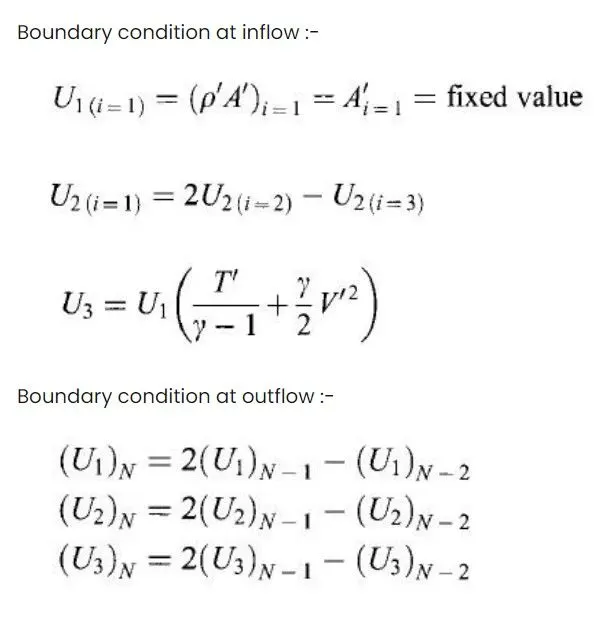
Boundary conditions for conservative scheme:
Code for Non-conservative part: (Supplementary function code-1)
function[rho,v,T,M,P,m,v_th,rho_th,T_th,M_th,m_th,P_th] = mac_non_cons(n,x,dx,T,v,c,a,gamma,nt,dt,rho,th)

%Outer time loop
for q = 1:nt

    %Initialization
    rho_0 = rho;
    T_0 = T;
    v_0 = v;

    %predictor method
    for i = 2:(n-1)

        dv_dx_p = ((v(i+1)-v(i))/dx);
        dloga_dx_p = (log(a(i+1))-log(a(i)))/dx;
        drho_dx_p = (rho(i+1)-rho(i))/dx;
        dT_dx_p = ((T(i+1)-T(i))/dx);

        %momentum eqn
        drho_dt_p(i) = -rho(i)*dv_dx_p - rho(i)*v(i)*dloga_dx_p - v(i)*drho_dx_p;

        %continuity eqn
        dv_dt_p(i) = -v(i)*dv_dx_p - (1/gamma)*(dT_dx_p + (T(i)/rho(i))*drho_dx_p);

        %Energy eqn
        dT_dt_p(i) = -v(i)*dT_dx_p-(gamma-1)*T(i)*(dv_dx_p+v(i)*dloga_dx_p);


        %Solution update
        rho(i) = rho(i) + drho_dt_p(i)*dt;
        v(i) = v(i) + dv_dt_p(i)*dt;
        T(i) = T(i) + dT_dt_p(i)*dt;

    end


    %Corrector method

    for i = 2:(n-1)

        dv_dx_c = ((v(i)-v(i-1))/dx);
        dloga_dx_c = (log(a(i))-log(a(i-1)))/dx;
        drho_dx_c = (rho(i)-rho(i-1))/dx;
        dT_dx_c = ((T(i)-T(i-1))/dx);

        %momentum eqn
        drho_dt_c(i) = -rho(i)*dv_dx_c - rho(i)*v(i)*dloga_dx_c - v(i)*drho_dx_c;

        %continuity eqn
        dv_dt_c(i) = -v(i)*dv_dx_c - (1/gamma)*(dT_dx_c + (T(i)/rho(i))*drho_dx_c);

        %Energy eqn
        dT_dt_c(i) = -v(i)*dT_dx_c-(0.4)*T(i)*(dv_dx_c+v(i)*dloga_dx_c);


    end

    %Computing average
    drho_dt = (drho_dt_p + drho_dt_c)/2;
    dT_dt = (dT_dt_p + dT_dt_c)/2;
    dv_dt = (dv_dt_p + dv_dt_c)/2;

    %Computing final solution
    for i = 2:n-1
        rho(i) = rho_0(i) + drho_dt(i)*dt;
        v(i)= v_0(i) + dv_dt(i)*dt;
        T(i) = T_0(i) + dT_dt(i)*dt;

    end


    %Boundary conditions

    %Inlet
    v(1) = 2*v(2) - v(3);

    %Outlet
    v(n) = 2*v(n-1) - v(n-2);
    rho(n) = 2*rho(n-1) - rho(n-2);
    T(n) = 2*T(n-1) - T(n-2);

    %Mach number
    M = v./((T).^0.5);
    %mass
    m = rho.*a.*v;
    %Pressure
    P = rho.*T;


    %Parameters at throat section
    v_th(q) = v(th);
    rho_th(q) = rho(th);
    T_th(q) = T(th);
    M_th(q) = M(th);

    m_th(q) = m(th);
    P_th(q) = P(th);


    %Plotting variation of mass flow rate at different time steps
    figure(4)
    hold on
    if q==0
        plot(x,m,'linewidth',1.5,displayName=['timestep= ', num2str(q)])
        hold on
    elseif q==50
        plot(x,m,'linewidth',1.5,displayName=['timestep= ', num2str(q)])
        %         hold on
    elseif q == 100
        plot(x,m,'linewidth',1.5,displayName=['timestep= ', num2str(q)])
        %         hold on
    elseif q == 150
        plot(x,m,'linewidth',1.5,displayName=['timestep= ', num2str(q)])
        %         hold on
    elseif q == 200
        plot(x,m,'linewidth',1.5,displayName=['timestep= ', num2str(q)])
        %         hold on
    elseif q==700
        plot(x,m,'linewidth',1.5,displayName=['timestep= ', num2str(q)])
        %         hold on
    elseif q == 1400
        plot(x,m,'linewidth',1.5,displayName=['timestep= ', num2str(q)])
        %         hold on
        xlabel('distance')
        ylabel('mass flow rate')
        title('Variation of mass flow rate at different time steps- Non conservative approach')
        legend
        grid on
    end

end
end
Explanation:
- The inputs which are required to find the final output variables of non-conservative scheme are entered in the function with name 'mac_non_cons' in the right hand side of the equation.
- The outputs required for non conservative scheme such as density, velocity, temperature, mach number, pressure and mass at all the section of the nozzle and also at throat section are needed to computed which is written in the left side of the function equation.
- First a outer time 'for' loop is inserted and then inner space 'for' loop is inserted to find the variables at each section of the nozzle. Then these variables at each section has to be determined for each time step until converges to the final solution.
- Then initial values of density, temperature and velocity are assigned at the start of the time loop.
- Using Macormack method, first step of predictor method is proceeded where the governing continuity, momentum and energy equation are to be determined using 'Forward differencing scheme'.
- Then solution has to be updated by summing the previous initial values of variables with the obtained forward differencing time derivatives. Then the space loop is ended.
- Next comes the corrector method where the same procedure is repeated but with 'Backward differencing scheme' to find the time derivatives of the variables at all section of the nozzle.
- Then the average of predictor and corrector has to be found and final solution is computed by summing up the initial values of the variables and the average values of the derivatives of predictor and corrector in the form of 'for' loop and then loop is ended.
- Before going to the next time step, the boundary conditions are entered by taking linear extrapolation at inlet and outlet points.
- Using the variables (velocity, temperature and density), the Mach number, mass flow rate and pressure has to be found using the formulas mentioned above.
- Then the parameters has to be determined at the throat section also by finding values at minimum area of the nozzle and then updated.
- Then the plotting of mass flow rate at different time steps is done and the time loop is ended which carries iteration for next time loop.
Code for Conservative part: (Supplementary function code-2)
function[rho,v,T,P,M,m,rho_th,v_th,T_th,P_th,M_th,m_th] = mac_cons(n,x,dx,a,v,U1,U2,U3,nt,dt,F1,F2,F3,rho,T,gamma,th)


%Macormack's technique
%Predictor method

for q = 1:nt

    %Initialization
    rho_0 = rho;
    T_0 = T;
    v_0 = v;

    U1_0 = U1;
    U2_0 = U2;
    U3_0 = U3;

    F1 = U2;
    F2 = (U2.^2./U1) + ((gamma-1)/gamma).*(U3-(gamma/2).*(U2.^2./U1));
    F3 = gamma.*((U2.*U3)./U1) - (gamma*(gamma-1)/2).*(U2.^3./U1.^2);

    for j = 2:n-1
        dF1_dx_p(j) = (F1(j+1)-F1(j))/dx;
        dF2_dx_p(j) = (F2(j+1)-F2(j))/dx;
        dF3_dx_p(j) = (F3(j+1)-F3(j))/dx;
        J2 = (1/gamma)*rho(j)*T(j)*(a(j+1)-a(j))/dx;

        %Continuity equation
        dU1_dt_p(j) = -(dF1_dx_p(j));
        dU2_dt_p(j) = -dF2_dx_p(j) + J2;
        %   ((gamma-1)/gamma).*(U3(j)-(gamma/2).*(U2(j).^2./U1(j)).*((log(a(j+1))-log(a(j)))/dx));

        dU3_dt_p(j) = -dF3_dx_p(j);

        %Solution update
        U1(j) = U1(j) + dU1_dt_p(j)*dt;
        U2(j) = U2(j) + dU2_dt_p(j)*dt;
        U3(j) = U3(j) + dU3_dt_p(j)*dt;

    end

    %Corrector

    F1 = U2;
    F2 = (U2.^2./U1) + ((gamma-1)/gamma).*(U3-(gamma/2).*(U2.^2./U1));
    F3 = gamma.*((U2.*U3)./U1) - (gamma*(gamma-1)/2).*(U2.^3./U1.^2);

    for j = 2:n-1
        dF1_dx_c(j) = (F1(j)-F1(j-1))/dx;
        dF2_dx_c(j) = (F2(j)-F2(j-1))/dx;
        dF3_dx_c(j) = (F3(j)-F3(j-1))/dx;

        J2 = (1/gamma)*rho(j)*T(j)*(a(j)-a(j-1))/dx;

        %Continuity equation
        dU1_dt_c(j) = -(dF1_dx_c(j));
        dU2_dt_c(j) = -dF2_dx_c(j) + J2;
        %((gamma-1)/gamma).*(U3(j)-(gamma/2).*(U2(j).^2./U1(j)).*((log(a(j))-log(a(j-1)))/dx));
        dU3_dt_c(j) = -dF3_dx_c(j);


    end


    %Computing average
    dU1_dt_avg = 0.5*(dU1_dt_p + dU1_dt_c);
    dU2_dt_avg = 0.5*(dU2_dt_p + dU2_dt_c);
    dU3_dt_avg = 0.5*(dU3_dt_p + dU3_dt_c);

    %Computing final solution
    for i = 2:n-1
        U1(i) = U1_0(i) + dU1_dt_avg(i).*dt;
        U2(i) = U2_0(i) + dU2_dt_avg(i).*dt;
        U3(i) = U3_0(i)+ dU3_dt_avg(i).*dt;

    end


    %Boundary conditions

    %Boundary conditions for sub-sonic inflow
    U1(1) = a(1);
    U2(1) = 2*U2(2)-U2(3);
    U3(1) = U1(1).*(T(1)/(gamma-1) + (gamma/2).*v(1).^2);

    %Boundary conditions for supersonic outflow
    U1(n) = 2*(U1(n-1)) - (U1(n-2));
    U2(n) = 2*(U2(n-1)) - (U2(n-2));
    U3(n) = 2*(U3(n-1)) - (U3(n-2));

    %Recomputing th primitive variables
    rho = U1./a;
    v = U2./U1;
    T = (gamma-1)*((U3./U1) - (gamma/2).*v.^2);
    P = rho.*T;

    %Mach number
    M = v./(sqrt(T));
    %mass
    m = rho.*a.*v;


    %Parameters at throat section
    v_th(q) = v(th);
    rho_th(q) = rho(th);
    T_th(q) = T(th);
    M_th(q) = M(th);

    m_th(q) = m(th);
    P_th(q) = P(th);


    %Plotting variation of mass flow rate at different time steps
    figure(5)
    if q==0
        plot(x,m,'linewidth',1.5,displayName=['timestep= ', num2str(q)])
        hold on
    elseif q==50
        plot(x,m,'linewidth',1.5,displayName=['timestep= ', num2str(q)])
        hold on
    elseif q == 100
        plot(x,m,'linewidth',1.5,displayName=['timestep= ', num2str(q)])
        hold on
    elseif q == 150
        plot(x,m,'linewidth',1.5,displayName=['timestep= ', num2str(q)])
        hold on
    elseif q == 200
        plot(x,m,'linewidth',1.5,displayName=['timestep= ', num2str(q)])
        hold on
    elseif q==700
        plot(x,m,'linewidth',1.5,displayName=['timestep= ', num2str(q)])
        hold on
    elseif q == 1400
        plot(x,m,'linewidth',1.5,displayName=['timestep= ', num2str(q)])
        hold on
        xlabel('distance')
        ylabel('mass flow rate')
        title('Variation of mass flow rate at different time steps- conservative approach')
        legend
        grid on
    end


end
end
Explanation:
- The Macormack technique for conservative part is slightly different from non-conservative where the flux terms are written in the form of solution terms.
- The outputs entered are same as that of non-conservative form in 'function' equation and corresponding inputs are entered in the right side of the equation.
- First time 'for' loop is initialized, then the Machormack technique is implemented using predictor and corrector method and the boundary conditions are inplemented. Then the procedure is same as above non-conservative part.
Main code:
clear all
close all
clc

%NON-CONSERVATIVE FORM

%inputs
n = 31;
x = linspace(0,3,n);
dx = x(2)-x(1);

rho = 1-.3146.*x;
T = 1-.2314.*x;
v = (0.1+1.09*x).*T.^0.5;

%area
a = 1+2.2.*(x-1.5).^2;

%Throat section
% th = min(a);
th = find(a==min(a));

%CFL number
c = 0.5;

%gamma
gamma = 1.4;

%time step
nt = 1400;

%Computing time interval
dt_0 = c.*dx./((sqrt(T))+v);
dt = min(dt_0);

tic
[rho_nc, vel_nc, T_nc, M_nc, P_nc, m_nc, v_th_nc, rho_th_nc, T_th_nc, M_th_nc, m_th_nc, P_th_nc] = mac_non_cons(n,x,dx,T,v,c,a,gamma,nt,dt,rho,th);
simulation_time_nc = toc


%%%%%%%%%%%%%%%%%%%%%

%CONSERVATIVE FORM

for i = 1:length(x)

    if x(i)>=0 && x(i)<=0.5
        rho(i) = 1;
        T(i) = 1;
    end

    if x(i)>=0.5 && x(i)<=1.5
        rho(i) = 1-0.366.*(x(i)-0.5);
        T(i) = 1-0.167.*(x(i)-0.5);
    end

    if x(i)>=1.5 && x(i)<=3.5
        rho(i) = 0.634-0.3879.*(x(i)-1.5);
        T(i) = 0.833-0.3507.*(x(i)-1.5);
    end

end
v = 0.59./(rho.*a);
U1 = rho.*a;
U2 = rho.*a.*v;
U3 = rho.*((T./(gamma-1))+(gamma/2).*(v.^2)).*a;

%Computing time interval
dt_0 = c.*dx./((sqrt(T))+v);
dt = min(dt_0);

%Writing flux vector in terms of solution vector
F1 = U2;
F2 = (U2.^2./U1) + ((gamma-1)/gamma).*(U3-(gamma/2).*(U2.^2./U1));
F3 = gamma.*((U2.*U3)./U1) - (gamma*(gamma-1)/2).*(U2.^3./U1.^2);

tic
[rho_c,vel_c,T_c,Pr_c,M_c,m_c,rho_th_c,v_th_c,T_th_c,P_th_c,M_th_c,m_th_C] = mac_cons(n,x,dx,a,v,U1,U2,U3,nt,dt,rho,F1,F2,F3,T,gamma,th);
simulation_time_c = toc

%plotting

figure(1)
%plotting variables wrt distance
subplot(4,1,1)
plot(x,vel_nc,'linewidth',1.5);
hold on
plot(x,vel_c,'*');
legend('Non-conservative','conservative');
xlabel('distance');
ylabel('velocity');
title('Change in velocity w.r.t distance');
grid minor

subplot(4,1,2)
plot(x,rho_nc,'linewidth',1.5);
hold on
plot(x,rho_c,'*');
legend('Non-conservative','conservative');
xlabel('distance');
ylabel('density');
title('Change in density w.r.t distance');
grid minor

subplot(4,1,3)
plot(x,T_nc,'linewidth',1.5);
hold on
plot(x,T_c,'*');
legend('Non-conservative','conservative');
xlabel('distance');
ylabel('temperature');
title('Change in temperature w.r.t distance');
grid minor

subplot(4,1,4)
plot(x,M_nc,'linewidth',1.5);
hold on
plot(x,M_c,'*');
legend('Non-conservative','conservative');
xlabel('distance');
ylabel('Mach number');
title('Change in Mach number w.r.t distance');
grid minor


%plotting parameters wrt number of iterations

figure(3)

subplot(4,1,1)
plot(linspace(1,nt,nt),v_th_nc,'linewidth',1.5);
hold on
plot(linspace(1,nt,nt),v_th_c,'linewidth',1.5);
legend('Non-conservative','conservative');
xlabel('distance');
ylabel('velocity');
title('Change in velocity w.r.t iteration');
grid minor

subplot(4,1,2)
plot(linspace(1,nt,nt),T_th_nc,'linewidth',1.5);
hold on
plot(linspace(1,nt,nt),T_th_c,'linewidth',1.5);
legend('Non-conservative','conservative');
xlabel('distance');
ylabel('Temperature');
title('Change in Temperature w.r.t iteration');
grid minor

subplot(4,1,3)
plot(linspace(1,nt,nt),M_th_nc,'linewidth',1.5);
hold on
plot(linspace(1,nt,nt),M_th_c,'linewidth',1.5);
legend('Non-conservative','conservative');
xlabel('distance');
ylabel('Mach number');
title('Change in Mach number w.r.t iteration');
grid minor

subplot(4,1,4)
plot(linspace(1,nt,nt),rho_th_nc,'linewidth',1.5);
hold on
plot(linspace(1,nt,nt),rho_th_c,'linewidth',1.5);
legend('Non-conservative','conservative');
xlabel('distance');
ylabel('density');
title('Change in density w.r.t iteration');
grid minor

%plotting the variation of mass flow rate
figure(6)
plot(x,m_nc,'linewidth',1.5)
hold on
plot(x,m_c,'linewidth',1.5)
legend('Non-conservative','conservative');
xlabel('distance');
ylabel('Mass flow rate');
title('Change in non-dimensional variation in mass flow rate');
grid on
Explanation:
- Here, the inputs for the initial conditions are entered and the procedure is carried for 1400 time steps.
- The time interval is calculated using minimum time step approach and the velocity of sound is written in the non-dimensional form.
- Then the simulation time for non-conservative and conservative is carried by using tic and toc command.
- Finally the plots are plotted for variables with respect to distance, variables of the plot with respect to time step and the mass flow rate for both conservative and non-conservative and results are obtained as follows.
RESULTS (for 31 grid points):
1. Variation of mass flow rate at different time steps- non conservative approach
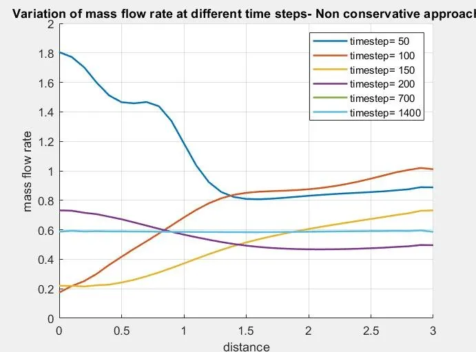
Observation:
- It is observe that as the time step increases, the variation of values nearly approaches to steady state.
- At 50th time step iteration, the value of mass flow rate changes from 1.8 to 0.8 in the sub sonic region and then approaches to steady state of 0.8.
- Then the variations dilutes slowly as the time step increases and at time step of 700th iteration, the value nearly approaches steady state of 0.6 and after 700th iteration the value shows nearly constant.
2. Variation of mass flow rate at different time steps- conservative approach
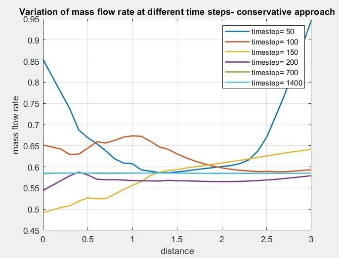
Observation:
- It is observe that as the time step increases, the variation of values nearly approaches to steady state.
- At 50th time step iteration, the value of mass flow rate changes from 0.85to 0.58 in the sub sonic region and then approaches to correct value near the sonic section then again value increases tin the super-sonic region.
- Then the variations dilutes slowly as the time step increases and at time step of 700th iteration, the value nearly approaches steady state of 0.85 and after 700th iteration the value shows nearly constant.
3. Change in parameters with respect to distance in the section:
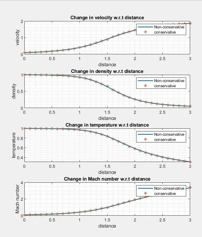
Observation:
- The values of non-conservative approach and the conservative approach are almost shows same results of parameters with respect to distance.
4. Change in parameters with respect to number of time steps:
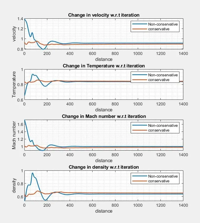
Observation:
- It is observed that conservative approach reaches the near to steady state value haster than non-conservative approach.
- The initial variation of the values is more in non-conservative approach than conservative.
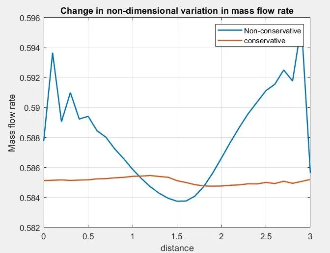
5. Change in non-dimensional variation in mass flow rate - at throat section:
Observation:
- At throat section, the conservative approach shows nearly constant results of 0.585 whereas non-conservative shows varied values across the section.
DISCUSSION:
- From the above it can be concluded that conservative approach are faster in converging results compared to non-conservative approach.
- Only silght differences in the values of primitive variables obtained for conservative and non-conservative for 31 grid points.
RESULTS (for 61 grid points, number of time steps=2800):
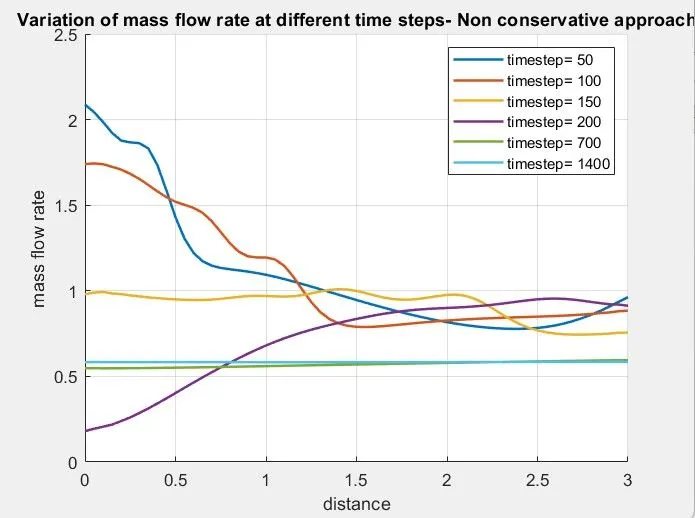
1. Variation of mass flow rate at different time steps- non conservative approach:
Observation:
- It is observed that as the time step increases, the variation of values nearly approaches to steady state.
- At 50th time step iteration, the value of mass flow rate changes from 2.1to 0.8.
- Then the variations dilutes slowly as the time step increases and at time step of 700th iteration, the value nearly approaches steady state of 0.6 and after 700th iteration the value shows nearly constant.
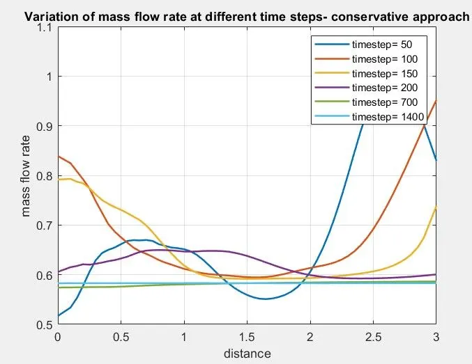
2. Variation of mass flow rate at different time steps- conservative approach:
Observation:
- It is observe that as the time step increases, the variation of values nearly approaches to steady state.
- At 50th time step iteration, the values are completely unsteady at initial range of time steps.
- Then the variations dilutes slowly as the time step increases and at time step of 700th iteration, the value nearly approaches steady state of 0.59 and after 700th iteration the value shows nearly constant.
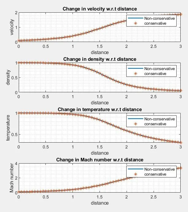
3. Change in parameters with respect to distance in the section:
Observation:
- The values of non-conservative approach and the conservative approach are almost shows same results of parameters with respect to distance.
4. Change in parameters with respect to number of time steps:
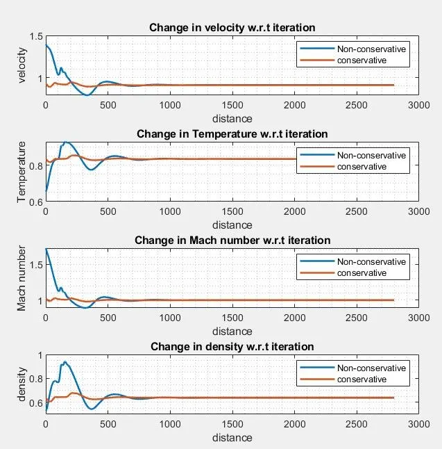
Observation:
- It is observed that conservative approach reaches the near to steady state value haster than non-conservative approach.
- The initial variation of the values is more in non-conservative approach than conservative.
5. Change in non-dimensional variation in mass flow rate - at throat section:
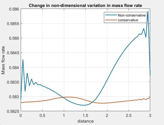
Observation:
- At throat section, the conservative approach shows nearly constant results of 0.582 whereas non-conservative shows varied values across the section.
DISCUSSION:
- From the above it can be concluded that conservative approach are faster in converging results compared to non-conservative approach.
- Differences in the final values of primitive variables obtained for conservative and non-conservative is negligible.
Grid independence test:
- Grid independence is achieved when the result of the plots remains same eventhough the number of grid point changes.
- In the above case, the experiment is performed for 31 and 61 number of grid points. When doubling the number of grid points, the number of iteration also to be doubled from 1400 to 2800.
- The values almost shows similar results which shows grid independency is achieved.
CONCLUSION:
- It is concluded that conservative form approaches to steady state at faster rate than non-conservative and deviation of results in conservative form are less from the steady state.
- The non conservative form deals directly with the primitive variables whereas in conservative form, the flux vectors are written in terms of solution vectors and then the method is proceeded. After getting results, again the solution vectors are converted into primitive variables which is a tideous process. So it takes more time for simulating since the number of steps are more in conservative than non conservative. So simulation time is less for non-conservative.
- Since the primitive variables are converted into solution variables and coding is proceeded and then reconverting again, there are possibilities of error since number of steps is more. So non-conservative part is more accurate and easy to code and less complex.
- For mass flow rate, conservative part gives better result since the value is almost constant across the section.