Week 3.5 - Deriving 4th order approximation of a 2nd order derivative using Taylor Table method

AIM:

• To

Derive the following 4th order approximations of the second-order derivative.

1. Central difference

2. Skewed right-sided difference

3. Skewed left-sided difference

• To write a program in Matlab to evaluate the second-order derivative of the analytical function exp(x)*cos(x) and compare it with the 3 numerical approximations
• To provide a plot that compares the absolute error between the above-mentioned schemes.

BODY OF CONTENT:

Taylor's method:

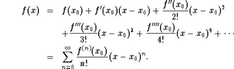
The Taylor series formula is the representation of any function as an infinite sum of terms. These terms are calculated from the values of the function’s derivatives at a single point. A function can be approximated by using a finite number of terms in its Taylor series. Taylor’s theorem is providing quantitative estimates on the error.

OBJECTIVE1:

Derive the following 4th order approximations of the second-order derivative.

1. Central difference

2. Skewed right-sided difference

3. Skewed left-sided difference

• Central difference :

The order of accuracy P = Number of nodes in the stencil N - order of derivative Q + 1 for symmetric/central schemes

Therefore, N = P+Q-1

Here P = 4, Q = 2

Therefore, Number of nodes in the stencil N = 5

Step1: The Taylor's series is derived for each nodes in the stencil in the central difference method. Since the number of nodes is taken as 5, so first 5 elements has to be considered in the Taylor's series as the main elements.

Taylor's table:

f'(x)*(Δx)n→ f’’(x)*(Δx)2↓	F(i)	f’(i)*(Δx)	f’’(i)*(Δx)2	f’’’(i)*(Δx)3	fIV(i)*(Δx)4	fV(i)*(Δx)^5	fVI(i)*(Δx)^6
a*f(i-2)	a	-2*a	2*a	-8*a/6	16*a/24	-32*a/30	64*a/720
b*f(i-1)	b	-b	b/2	-b/6	b/24	-b/20	b/720
c*f(i)	c	0	0	0	0	0	0
d*f(i+1)	d	d	d/2	d/6	d/24	d/20	d/720
e*f(i+2)	e	2*e	2*e	8*e/6	16*e/24	32*a/120	64*a/720
(ꝺ2 f/ ꝺx2)	0	0	1 (Desired one)	0	0	Don’t know	Don’t know

Step2: Finding constants a,b,c,d,e

Since the second order derivative is asked, it is necessary to equate the second order derivative to 1 and keeping the rest of the derivatives '0' in the Taylor's table coloumn. But the 5th and 6th derivative is unknown. So considering the first 5 elements in the Taylor's table, the equations are solved and constants are obtained.

The equations are obtained as given below from the Taylor's table.

a + b+ c+ d+ e =0 ...................(1)

-2a -b +0 +d +2e = 0 ...................(2)

2a +b/2 +0 +d/2 +2e = 1 ...................(3)

-8a/6 -b/6 +0 +d/6 +8e/6 =0 ...................(4)

16a/24 + b/24 + 0 +d/24 +16e/24 = 0 ..................(5)

The above equation has to be solved in the matrix form.

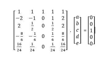
AX = B

To solve this matrix multiplication and to determine the 'X' values, it is done by MATLAB program using 'linsolve' command for matrix multiplication.

CODE:

close all
clear all
clc
 
%Central differencing scheme matrix multiplication.
A = [1 1 1 1 1; -2 -1 0 1 2; 2 1/2 0  1/2 2; -8/6 -1/6 0 1/6 8/6; 16/24 1/24 0 1/24 16/24];
B = [0; 0; 1; 0; 0];
x = linsolve(A,B)

The 'X' value is determined and the constants are found to be as shown.

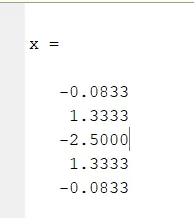
By Taylor's series using central difference scheme, the fourth order approximation for second order derivative is obtained as,

(ꝺ² f/ ꝺx²) = a*f(i-2) + b*f(i-1) + c*f(i) + d*f(i+1) + e*f(i+2)

a*f(i-2) + b*f(i-1) + c*f(i) + d*f(i+1) + e*f(i+2) = (a + b+ c+ d+ e)*F(i) + (-2a -b +0 +d +2e )*f’(i)*(Δx) + (2a +b/2 +0 +d/2 +2e )*f’’(i)*(Δx)² + (-8a/6 -b/6 +0 +d/6 +8e/6) *f’’’(i)*(Δx)³ + * + (16a/24 + b/24 + 0 +d/24 +16e/24) * f^IV(i)*(Δx)⁴+ (-32*a/30 -b/120 +0 +d/120 +32a/120 ) * f^V(i)*(Δx)^5 + (64a/720 +b/720 +0 +d/720 +64a/720)*f^VI(i)*(Δx)^6

The above are the equation obtained. Since we need the second order derivative we are approximating the other derivatives upto 4th order to 0. But the 5th order automatically cancels and becomes 0. So the left out equation is

[a*f(i-2) + b*f(i-1) + c*f(i) + d*f(i+1) + e*f(i+2) ]= [ (2a +b/2 +0 +d/2 +2e )*f’’(i)*(Δx)^2 + (64a/720 +b/720 +0 +d/720 +64a/720)*f^VI(i)*(Δx)^6 ]

(Dividing the equation by Δx²)

[a*f(i-2) + b*f(i-1) + c*f(i) + d*f(i+1) + e*f(i+2) ] / Δx² = f’’(x) + (64a/720 +b/720 +0 +d/720 +64a/720)*f^VI(i)*(Δx)^4

[a*f(i-2) + b*f(i-1) + c*f(i) + d*f(i+1) + e*f(i+2) ] / Δx² = f’’(x) + Truncation error of order 4.

where Truncation error of order 4 = (64a/720 +b/720 +0 +d/720 +64a/720) (approimated as 0)

Therefore,

.........(1)

• Skewed right-sided difference

The order of accuracy P = Number of nodes in the stencil N - order of derivative Q for one-sided/skewed schemes

N = P+Q

N = 4 + 2 =6

Therefore the number of nodes in the stencil to be considered is 6

The nodes are assumed as [f(i), f(i+1), f(i+2), f(i+3), f(i+4), f(i+5)]

From Taylor's series, we get the values of the above nodes are listed in the Taylor's table.

Taylor's table:

f'(x)*(Δx)n→ f’’(x)*(Δx)2↓	F(i)	f’(i)*(Δx)	f’’(i)*(Δx)2	f’’’(i)*(Δx)3	fIV(i)*(Δx)4	fV(i)*(Δx)^5	fVI(i)*(Δx)^6
a*f(i)	a	0	0	0	0	0	0
b*f(i+1)	b	b	b/2	b/6	b/24	b/120	b/720
c*f(i+2)	c	2c	4c/2	8c/6	16c/24	32c/120	64c/720
d*f(i+3)	d	3d	9d/2	27d/6	81d/24	243d/120	729d/720
e*f(i+4)	e	4e	16e/2	64e/6	256e/24	1024e/120	4096e/720
g*f(i+5)	g	5g	25g/2	125g/6	625g/24	3125e/120	15625g/720
(ꝺ2 f/ ꝺx2)	0	0	1	0	0	0	Don't know

Step2: Finding constants a,b,c,d,e

Since the second order derivative is asked, it is necessary to equate the second order derivative to 1 and keeping the rest of the derivatives '0' in the Taylor's table coloumn. But the 6th derivative is unknown. So considering the first 6 elements in the Taylor's table, the equations are solved and constants are obtained.

The equations are obtained as given below from the Taylor's table.

a + b+ c+ d+ e =0 ...................(1)

0 + b+ 2c+ 3d+ 4e+ 5g = 0 ...................(2)

0 +b/2 + 4c/2 +9d/2 +16e/2 +25g/2 = 1 ...................(3)

0 +b/6 +8c/6 +27d/6 + 64e/6 +125g/6 = 0 ...................(4)

0 +b/24 +16c/24 +81d/24 +256e/24 +625g/24 =0 ...................(5)

0 +b/120 +32c/120 +243d/120 +1024e/120 +3125g/120 = 0 ...................(6)

The above equation has to be solved in the matrix form.

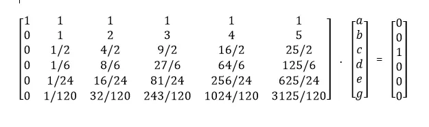
AX = B

To solve this matrix multiplication and to determine the 'X' values, it is done by MATLAB program using 'linsolve' command for matrix multiplication.

CODE:

%Skewed right sided difference scheme
A1 = [1 1 1 1 1 1; 0 1 2 3 4 5; 0 1/2 4/2 9/2 16/2 25/2 ; 0 1/6 8/6 27/6 64/6 125/6; 0 1/24 16/24 81/24 256/24 625/24; 0 1/120 32/120 243/120 1024/120 3125/120];
B1 = [0; 0; 1; 0; 0; 0];
x1 = linsolve(A1,B1)

The 'X' value is determined and the constants are found to be as shown.

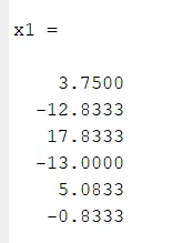
By Taylor's series using skewed right sided scheme, the fourth order approximation for second order derivative is obtained as,

(ꝺ² f/ ꝺx²) = a*f(i) + b*f(i+1) + c*f(i+2) + d*f(i+3) + e*f(i+4) + g*f(i+5)

Since we need the second order derivative we are approximating the other derivatives upto 5th order to 0 except second order derivative which is equated to 1.

Similar to previous central differencing, by solving the above Taylors series we get solution as

which is the hypothesis of skewed right sided differencing for 4th order approximation for second order derivative.

• Skewed left-sided difference

The order of accuracy P = Number of nodes in the stencil N - order of derivative Q for one-sided/skewed schemes

N = P+Q

N = 4 + 2 =6

Therefore the number of nodes in the stencil to be considered is 6

The nodes are assumed as [f(i), f(i-1), f(i-2), f(i-3), f(i-4), f(i-5)]

From Taylor's series, we get the values of the above nodes are listed in the Taylor's table.

Taylor's table:

f'(x)*(Δx)n→ f’’(x)*(Δx)2↓	F(i)	f’(i)*(Δx)	f’’(i)*(Δx)2	f’’’(i)*(Δx)3	fIV(i)*(Δx)4	fV(i)*(Δx)^5	fVI(i)*(Δx)^6
a*f(i)	a	0	0	0	0	0	0
b*f(i+1)	b	-b	b/2	-b/6	b/24	-b/120	b/720
c*f(i+2)	c	-2c	4c/2	-8c/6	16c/24	-32c/120	64c/720
d*f(i+3)	d	-3d	9d/2	-27d/6	81d/24	-243d/120	729d/720
e*f(i+4)	e	-4e	16e/2	-64e/6	256e/24	-1024e/120	4096e/720
g*f(i+5)	g	-5g	25g/2	-125g/6	625g/24	-3125e/120	15625g/720
(ꝺ2 f/ ꝺx2)	0	0	1	0	0	0	Don't know

Step2: Finding constants a,b,c,d,e

Since the second order derivative is asked, it is necessary to equate the second order derivative to 1 and keeping the rest of the derivatives '0' in the Taylor's table coloumn. But the 6th derivative is unknown. So considering the first 6 elements in the Taylor's table, the equations are solved and constants are obtained.

The equations are obtained as given below from the Taylor's table.

a + b+ c+ d+ e =0 ...................(1)

0 - b- 2c- 3d- 4e- 5g = 0 ...................(2)

0 +b/2 + 4c/2 +9d/2 +16e/2 +25g/2 = 1 ...................(3)

0 -b/6 -8c/6 -27d/6 - 64e/6 -125g/6 = 0 ...................(4)

0 +b/24 +16c/24 +81d/24 +256e/24 +625g/24 =0 ...................(5)

0 -b/120 -32c/120 -243d/120 -1024e/120 -3125g/120 = 0 ...................(6)

The above equation has to be solved in the matrix form.

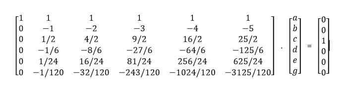
AX = B

To solve this matrix multiplication and to determine the 'X' values, it is done by MATLAB program using 'linsolve' command for matrix multiplication.

CODE:

%Skewed left sided difference scheme
A2 = [1 1 1 1 1 1; 0 -1 -2 -3 -4 -5; 0 1/2 4/2 9/2 16/2 25/2 ; 0 -1/6 -8/6 -27/6 -64/6 -125/6; 0 1/24 16/24 81/24 256/24 625/24; 0 -1/120 -32/120 -243/120 -1024/120 -3125/120];
B2 = [0; 0; 1; 0; 0; 0];
x2 = linsolve(A1,B1)

The 'X' value is determined and the constants are found to be as shown.

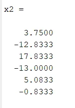
By Taylor's series using skewed left sided scheme, the fourth order approximation for second order derivative is obtained as,

(ꝺ² f/ ꝺx²) = a*f(i) + b*f(i-1) + c*f(i-2) + d*f(i-3) + e*f(i-4) + g*f(i-5)

Since we need the second order derivative we are approximating the other derivatives upto 5th order to 0 except second order derivative which is equated to 1.

Similar to previous differencing schemes, by solving the above Taylors series we get solution as

Matlab to evaluate the second-order derivative of the analytical function exp(x)*cos(x) and compare it with the 3 numerical approximations:

close all
clear all
clc

%f = exp(x)*cos(x)
%second derivative of f = -2*exp(x)*sin(X)
% assume x=pi/6
 x = pi/6
analytical_val = -2*exp(x)*sin(x)

%range of dx values
dx = linspace(pi/3000,pi/3,50);


for i = 1:length(dx)
%second derivative using central difference scheme
cen_diff(i) = (-0.0833*exp(x-2*dx(i))*cos(x-2*dx(i))+1.3333*exp(x-dx(i))*cos(x-dx(i))-2.5*exp(x)*cos(x)+1.3333*exp(x+dx(i))*cos(x+dx(i))-0.0833*exp(x+2*dx(i))*cos(x+2*dx(i)))/(dx(i))^2;

%second derivative using skewed right sided scheme
right_skew(i) = (3.75*exp(x)*cos(x)-12.8333*exp(x+dx(i))*cos(x+dx(i))+17.8333*exp(x+2*dx(i))*cos(x+2*dx(i))-13*exp(x+3*dx(i))*cos(x+3*dx(i))+5.0833*exp(x+4*dx(i))*cos(x+4*dx(i))-0.8333*exp(x+5*dx(i))*cos(x+5*dx(i)))/(dx(i))^2 ;

%second derivative using skewed left scheme
left_skew(i) = (3.75*exp(x)*cos(x)-12.8333*exp(x-dx(i))*cos(x-dx(i))+17.8333*exp(x-2*dx(i))*cos(x-2*dx(i))-13*exp(x-3*dx(i))*cos(x-3*dx(i))+5.0833*exp(x-4*dx(i))*cos(x-4*dx(i))-0.8333*exp(x-5*dx(i))*cos(x-5*dx(i)))/(dx(i))^2 ;


%error measurement
error_cen(i) = abs(cen_diff(i) - analytical_val)

error_left(i) = abs(left_skew(i) - analytical_val)

error_right(i) = abs(right_skew(i) - analytical_val)


end


%plotting
figure(1)
plot(dx,error_cen,dx,error_left,dx,error_right,'linewidth',2);
legend('central difference','Right skewed','left skewed');
title('Error comparision for three schemes')
xlabel('step size(dx)')
ylabel('error')

figure(2)
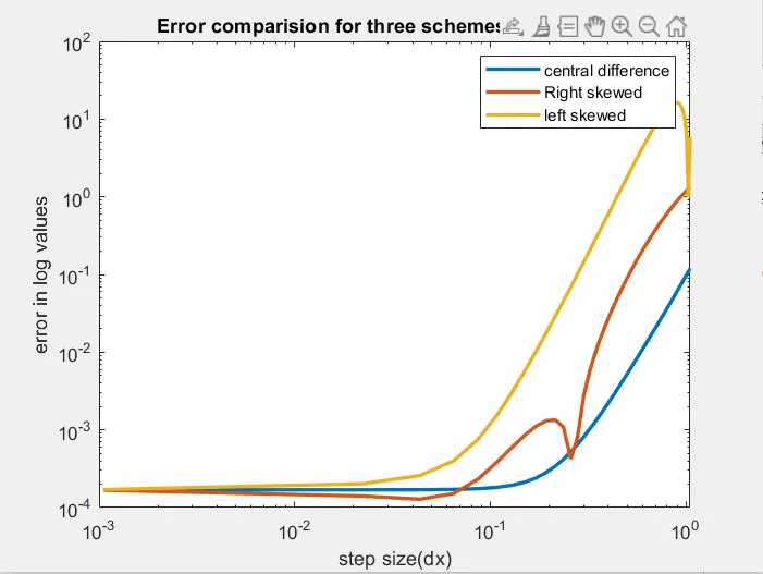
loglog(dx,error_cen,dx,error_left,dx,error_right,'linewidth',2)
legend('central difference','Right skewed','left skewed')
title('Error comparision for three schemes in log values')
xlabel('step size(dx)')
ylabel('error in log values')

Explanation:

Here, the analytical value for the given function for second order derivative is found first. Then second order derivative for the 3 schemes is found using the formula derived above for the step size ranging from pi/3000 to pi/3 taking 49 intervals inbetween using 'linspace' command and assuming 'x' value as pi/6.

After getting all the values in the given range for the 3 schemes, the error has to be compared with the analytical value of the second derivative using 'abs' command.

Finally, the error for the three schemes are plotted in graph for the given range and compared using 'plot' command. To magnify the plot, 'loglog' command is used which is used to plot in log values.

RESULT:

Error comparision:

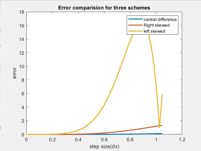
Error comparision in 'log' plot:

CONCLUSION FROM RESULT:

• From the graph, it is found out that mean slope of the left skewed scheme is highest among all, next comes right skewed scheme and Central difference scheme has the least slope of error as the step size increases.
• At the beginning, the right sided skewed scheme has negative slope for certain range. After that the rate of change of slope is high. So the right sided skewed scheme shows better results for small step size range where error is minimum.
• On overall aspect for the given function, the central difference scheme shows better result producing minimum error on average for the large range of step size values and gives good results for high step size values.
• The variation of error for any step size values for central differencing scheme is almost same and thus show approximately linear plot.
• The large error values for skewed schemes is due number of nodes is more (5) and for central differencing scheme, it is 2 only.
• For all the schemes, as the step size is more the error is more. So for accuracy to be maintained step size should be small.

Describe why a skewed scheme is useful? What can a skewed scheme do that a CD scheme cannot?

Skewed scheme is unconditionally bounded and highly stable but only first order accurate whereas central differencing scheme is 2nd order accurate in terms of truncation error but it is not always advisable to use central differencing scheme. In cases of one dimensional heat conduction applications like heat conduction/ heat transfer at the end of concrete wall and fins the heat is transfered from one end. So the we are restricted to use grid points from one side only. In such cases, we use skewed approximation and in this case central differencing is not advisable which has grid points at both sides.