Week 4 - CHT Analysis on Exhaust port
AIM:
To answer the following questions
- Give a brief description of why and where a CHT analysis is used.
- Maintain the y+ value according to the turbulence model and justify the results.
- Calculate the wall/surface heat transfer coefficient on the internal solid surface & show the velocity & temperature contours in appropriate areas.
- How would you verify if the HTC predictions from the simulations are right? On what factors does the accuracy of the prediction depend on?
SOLUTION:
CHT analysis:
The Conjugate Heat Transfer (CHT) analysis type allows for the simulation of heat transfer between solid and fluid domains by exchanging thermal energy at the interfaces between them. This type of heat transfer includes both convection (between fluids) and conductive (between solids) heat transfer, as well as both forced and natural convection.
Common applications and use cases of this thermal simulation type include electronics cooling, heat exchangers, industrial machinery, some AEC cases, and more.
The CHT approach has an advantage over FE thermal analyses in that wall heat transfer coefficients and their local variations on surfaces are directly calculated within the model rather than based on simplified empirical calculations. The CHT approach therefore has benefits for those applications where heat transfer is either non-uniform or difficult to calculate empirically. Heat sinks are optimized to combine heat transfer by conduction in the heat sink with the convection in the surrounding fluid.
Heat Transfer in a Solid
In most cases, heat transfer in solids, if only due to conduction, is described by Fourier’s law defining the conductive heat flux, q, proportional to the temperature gradient:  .
.
For a time-dependent problem, the temperature field in an immobile solid verifies the following form of the heat equation:

Heat Transfer in a Fluid
Due to the fluid motion, three contributions to the heat equation are included:
- The transport of fluid implies energy transport too, which appears in the heat equation as the convective contribution. Depending on the thermal properties on the fluid and on the flow regime, either the convective or the conductive heat transfer can dominate.
- The viscous effects of the fluid flow produce fluid heating. This term is often neglected, nevertheless, its contribution is noticeable for fast flow in viscous fluids.
- As soon as a fluid density is temperature-dependent, a pressure work term contributes to the heat equation. This accounts for the well-known effect that, for example, compressing air produces heat.
Accounting for these contributions, in addition to conduction, results in the following transient heat equation for the temperature field in a fluid:

Efficiently combining heat transfer in fluids and solids is the key to designing effective coolers, heaters, or heat exchangers.
The fluid usually plays the role of energy carrier on large distances. Forced convection is the most common way to achieve high heat transfer rate. In some applications, the performances are further improved by combining convection with phase change (for example liquid water to vapor phase change).
Even so, solids are also needed, in particular to separate fluids in a heat exchanger so that fluids exchange energy without being mixed.
Heat sinks are usually made of metal with high thermal conductivity (e.g. copper or aluminum). They dissipate heat by increasing the exchange area between the solid part and the surrounding fluid.
Energy Savings
Heat transfer in fluids and solids can also be combined to minimize heat losses in various devices. Because most gases (especially at low pressure) have small thermal conductivities, they can be used as thermal insulators… provided they are not in motion. In many situations, gas is preferred to other material due to its low weight. In any case, it is important to limit the heat transfer by convection, in particular by reducing the natural convection effects. Judicious positioning of walls and use of small cavities helps to control the natural convection. Applied at the micro scale, the principle leads to the insulation foam concept where tiny cavities of air (bubbles) are trapped in the foam material (e.g. polyurethane), which combines high insulation performances with light weight.
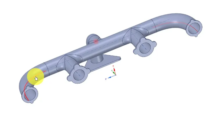
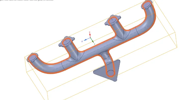
- The red enclosure is the fluid volume enclosure.
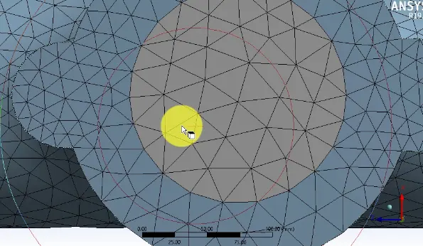
- Here, the fluid volume and solid volume are separate parts and are called non-conformal mesh. So to make a conformal, both fluid volume and solid volume should share the same boundary of mesh for smooth heat transfer. This is done by using share topology.
- To make this go to geometry, right click the fluid and solid volume and move it to the new component.
- Now right click 'fff' and delete empty component. Then click on 'fff component' and make share topology.
- Then go to prepare and select shareprep (or share and select the body and tick mark it).
- Now go to mesh and check the conformal mesh is seen without any interference.
Conformal mesh:
- Then create named selection for inlet, outlet and cylinder walls.
- Then update the mesh after checking the number of cells that can be fit for the present software to proceed simulation and open setup.
- Go to bounaries. Change inlet velocity to 5 m/s and inlet temperature to 700 degree celcius.
- In the boundary condition, click outer wall convection and select the heat transfer coefficient as 20 which is the value taken from experiments.
- Now initialize the case and go to solution and select contour and enter temperature contour after selecting the required wall regions for which the contours are required. Click save and display.
- Model : k-ω model (since the results are required near the wall boundary region)
Results:
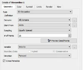
- Then go to results and open the solid post. Go to solid wall and color the variable with respect to temperature. Go to streamlines in the result toolbar and select the streamline to start from the inlet variable to display streamline for the flow pattern.
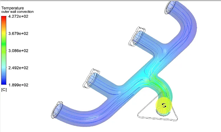
- Now insert the plane where the flow pattern and heat transfer co-efficient are to be analysed.
- Looking at the image above, we need to be careful to ensure that our y+ values are not so large that the first node falls outside the boundary layer region.
- If this happens, then the Wall Functions used by our turbulence model may incorrectly calculate the flow properties at this first calculation point which will introduce errors into our pressure drop and velocity results. The upper range of applicability will vary depending on the flow physics and the extent of the boundary layer profile.
Wall spacing calculation:
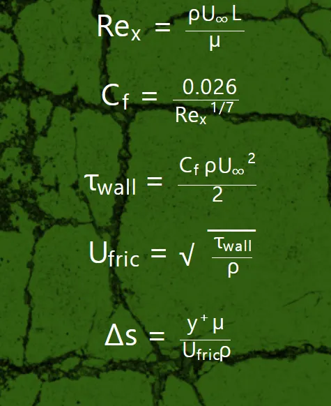 `tau`
`tau`Usually, for turbulance model the y+ value should be in the range of 0.1 to 5. In our case let us consider y+ value to be 1, Free stream velocity to be 5 m/s, density of air = 1.225 kg/m^3, D= 0.1662m (diameter of the inlet port) and dynamic viscosity = 0.000017894 Ns/m. After calculating from the parameters, the following results are obtained.
y+ = 1
Re = 56889.180730971275
△s = 0.00005601116952490746 <----[wall spacing]
3. Calculate the wall/surface heat transfer coefficient on the internal solid surface & show the velocity & temperature contours in appropriate areas:
Refined simulation of 20 mm mesh size:
Element size = 150 mm
Sizing element size = 20 mm
No of elements: 254008
Viscous model: k-ω model
Inlet velocity: 5 m/s
Inlet temperature: 700K
HTC : 20 W/(m^2-K)
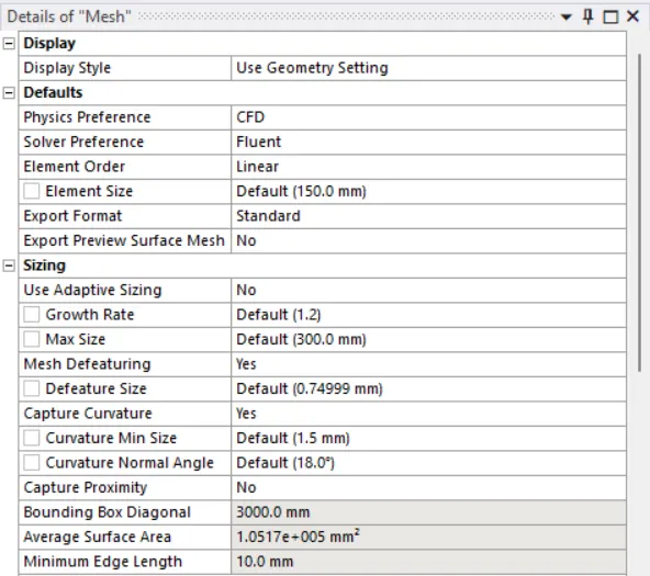

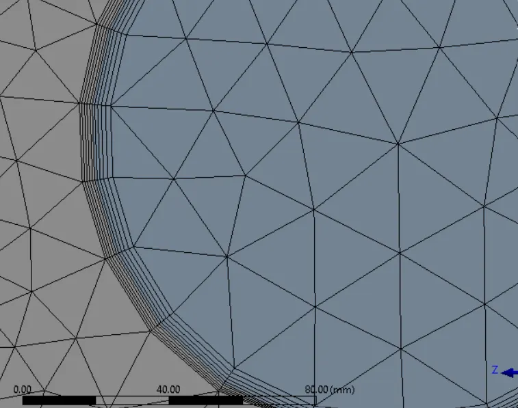
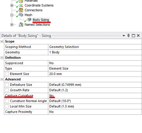
Enable capture the curvature:
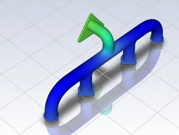
Temperature contour:
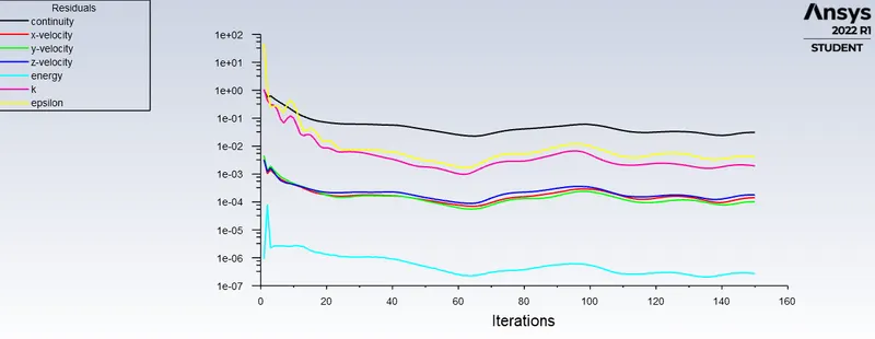
Residuals plot:
Heat transfer coefficient plot:
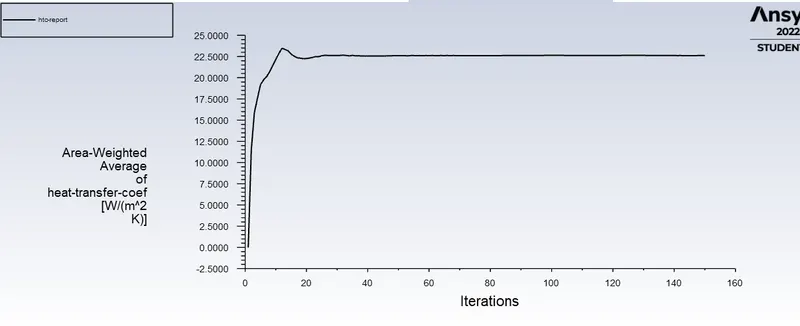
Temperature of the body surface plot:
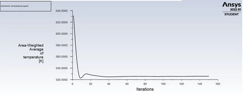
Reference values:
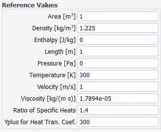
Heat transfer co-efficient value:

Temperature of the wall surface:

Total surface heat flux:

Velocity contour plot :
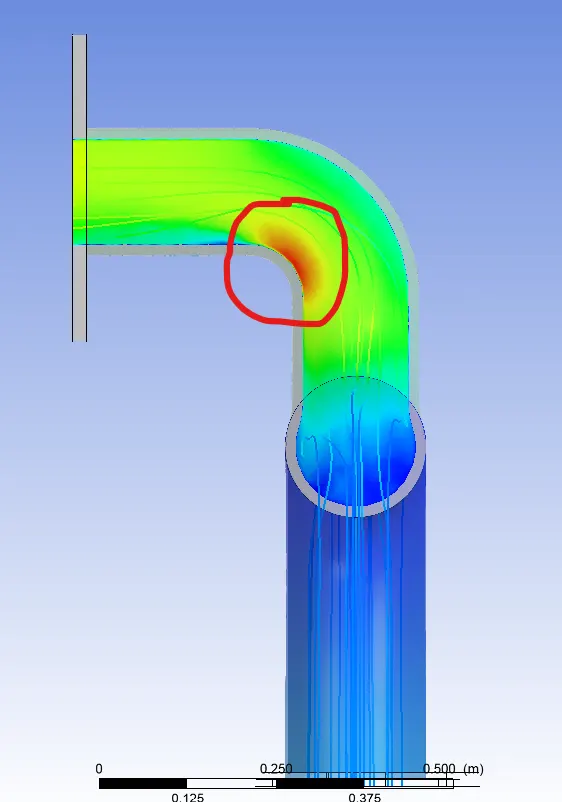
Temperature contour plot:
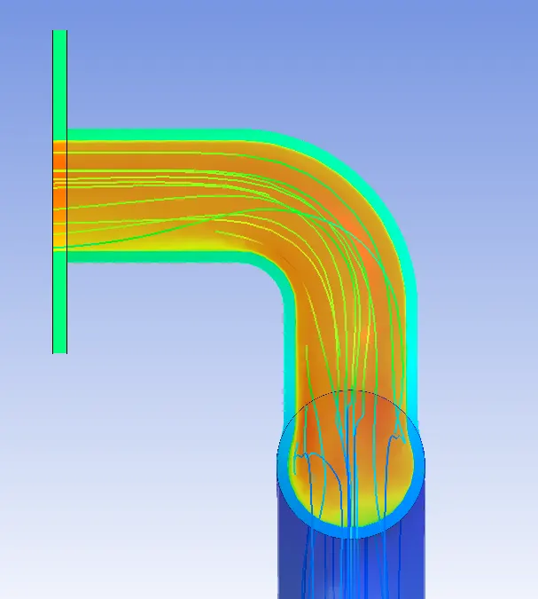
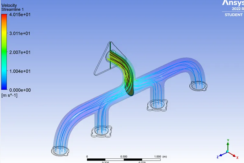
Streamlined plot:
4. How would you verify if the HTC predictions from the simulations are right? On what factors does the accuracy of the prediction depend on?
Analytical heat transfer co-efficient calculation:
- So from the above simulations we can conclude that the heat transfer coefficient is high near the curvature of the exhaust port because the temperature of the exhaust port near the bend is high which is due to turbulence effect near the bend increasing the velocity thus increasing the Reynold's number.
- The accuracy of the prediction depends upon the following factors of specific heat value, dynamic viscosity value, thermal conductivity value which are all taken as constant in analytical calculation but these values are sensitive withe respect to temperature though the values doesn't change to larger extent. So there is negligible difference in heat transfer co-efficient accuracy.
- Also the y+ value plays a major role in htc accuracy which the viscous sub layer thickness assumption should match with the actual thickness value.