Week 9 - FVM Literature Review
AIM:
- To describe Finite Volume Method(FVM) and the major differences between FDM & FVM.
- To describe the need for interpolation schemes and flux limiters in FVM.
SOLUTION:
Finite Volume Method(FVM):
FVM is in common use for discretizing computational fluid dynamics equations. The finite volume method (FVM) is a discretization technique for partial differential equations, especially those that arise from physical conservation laws. The finite volume method is a numerical method for solving partial differential equations that calculates the values of the conserved variables averaged across the volume. FVM uses a volume integral formulation of the problem with a finite partitioning set of volumes to discretize the equations.
Advantages of FVM:
- One advantage of the finite volume method over finite difference methods is that it does not require a structured mesh (although a structured mesh can also be used).
- Furthermore, the finite volume method is preferable to other methods as a result of the fact that boundary conditions can be applied noninvasively. This is true because the values of the conserved variables are located within the volume element, and not at nodes or surfaces.
- Finite volume methods are especially powerful on coarse nonuniform grids and in calculations where the mesh moves to track interfaces or shocks.
-
FVM is the ideal method for computing discontinuous solutions arising in compressible flows. Any discontinuity must satisfy the Rankine-Hugoniot jump condition which is a consequence of conservation. Since finite volume methods are conservative they automatically satisfy the jump conditions and hence give physically correct weak solutions.
FVM is also preferred while solving partial differential equations containing discontinuous coefficients.
- All these codes use midpoint-rule approximation for surface and volume integrals – so they are at most 2nd-order accurate. Approximations of gradients are also at most of 2nd-order.
Drawbacks of FDM:
- Method is suitable for 1-dimensional mesh with uniform grid spacing which gives proper results. But for 2-dimensional and 3-dimensional case with non-uniform grid spacing, Finite difference method is not suitable one. Here we use Finite Volume scheme as a best suitable option.
If we use Finite difference scheme for 2-D or 3-D structured mesh with non-uniform grid spacing, the correction process is done by variable approach method where it seeks to create grid in a variable space that looks in the form of cartesian grid. Instead, the nonuniform grid must (somehow) be transformed into a uniform, rectangular grid. Moreover, along with this transformation, the governing partial differential equations must be recast so as to apply in this transformed, rectangular grid with new coordinate lines 'ε' and 'η' are defined.
Example: - Assume we wish to calculate the flow over an airfoil, as sketched in Figure, , we have placed the airfoil in a rectangular grid.
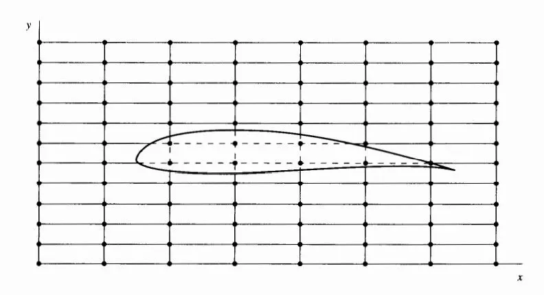
1. Some grid points fall inside the airfoil, where they are completely out of the flow.
2. There are few, if any, grid points that fall on the surface of the airfoil. This is not good, because the airfoil surface is a vital boundary condition for the determination of the flow, and hence the airfoil surface must be clearly and strongly seen by the numerical solution.
As a result, we can conclude that the rectangular grid in Figure above is not appropriate
for the solution of the flow field.
In contrast, a grid that is appropriate is sketched in Figure below. Here we see a nonuniform, curvilinear grid which is literally wrapped around the airfoil.
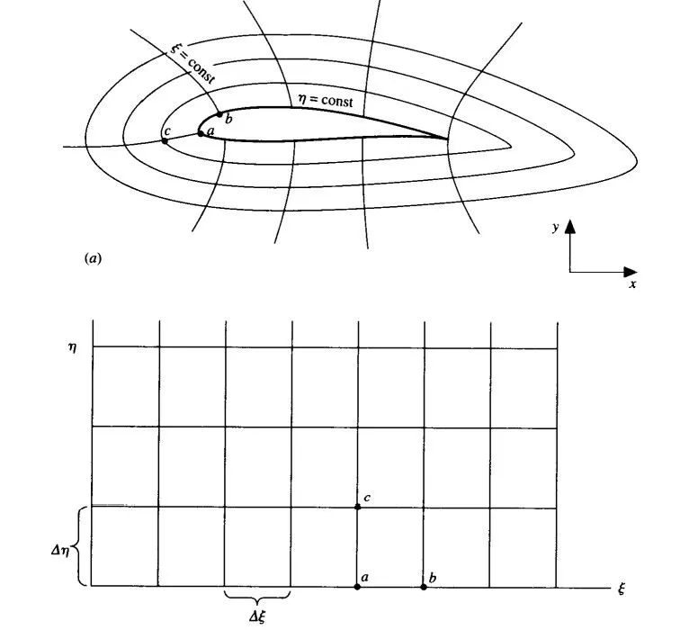
New coordinate lines 'ε' and 'η' are defined such that the airfoil surface becomes a coordinate line, 'η' = constant. This is called a boundary-fitted coordinate system.
The important point is that grid points naturally fall on the airfoil surface and grid is not rectangular and is not uniformly spaced. As a consequence, the conventional difference quotients are difficult to use. What must be done is to transform the curvilinear grid in physical space to a rectangular grid in terms of 'ε' and 'η'·
Moreover, when the governing equations are solved in the computational space, they must be expressed in terms of the variables 'ε' and 'η' rather than of x and y. That is, the governing equations must be transformed from (x, y) to ( 'ε' , 'η'·) as the new independent variables.
Again, the results are transformed from 'ε' and 'η' to 'x' and 'y' which is a complex task and it cannot be assured that the results will be correct and sometimes it is impossible to perform this in Finite difference method when the structure and mesh becomes very complex.
Major differences between FDM & FVM:
- FDM is suitable only for 1-D uniform spaced grids whereas FVM is suitable for both uniform and non-uniform grid spaced mesh.
- In FDM, whatever non-uniform grid exists in the physical space, there exist a transformation which will recast it as a uniform rectangular grid in the computational space. The FDM calculations are made over tis uniform grid in the computational space after which flow field results are transfered back to the corresponding points in the physical space.
Finite-volume calculations can be made directly in the physical plane on a nonuniform mesh. No transformations are necessary. Therefore, in the context of a finite-volume method, mesh generation simply involves the construction of the mesh in physical space. Finite volume method does not demand a uniform rectangular grids for compuations. - There is nothing about the finite-volume method that demands a structured mesh; it can be applied to mesh cells of any arbitrary shape. This allows for maximum flexibility in matching mesh cells with the boundary surfaces and for putting cells where you want them.
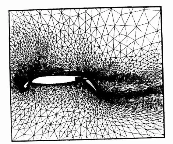
But for FDM we considered a cartesian grid, such as shown in the first figure above and then immediately rejected it for general use because of the difficulty posed by grid points appearing inside the body, as well as the lack of grid points on the boundary.
The mesh cells away from the body can be rectangular, and those cells adjacent to the body can be modified in shape such that one side of each cell is along the body surface. This is shown schematically in figure below.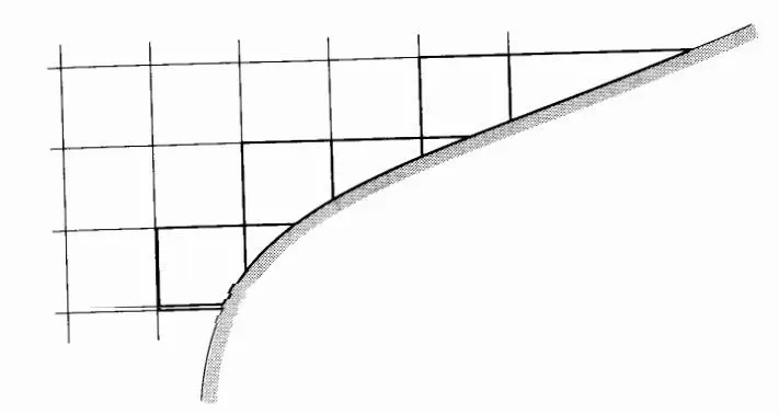
- Examples:
Finite-difference method: Weather calculations, astrophysics, seismology, physical realism in computer graphics, and special effects.
Finite-volume method: CFD, heat transfer, and chemical engineering.
- In Finite Differnece, the Dependant variable values are stored at the nodes only. But in FVM, the dependant values are stored in the center of the Finite volume.
- In FV approach, Conservation of mass, momentum, energy is ensured at each cell/finite volume level. This NOT true in FDM.
- FDM uses Taylor's series. FVM uses Gauss Divergence theorem.
- In FDM, properties are calculated for node basis. But in FVM, properties are calculated for cell basis instead of node.
Steps in FVM : (Considering 1D linear heat conduction equation as an example)
- The first step in the FVM is to divide the domain into a number of control volumes (aka cells, elements) where the variable of interest is located at the centroid of the control volume.
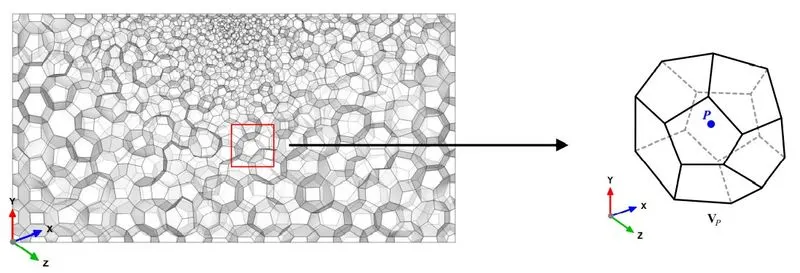
- The control volumes can be of any shape (e.g., tetrahedrons, hexes, prisms, pyramids, dodecahedrons, and so on). The only requirement is that the elements need to be convex and the faces that made up the control volume need to be planar.
- The next step is to integrate the differential form of the governing equations (very similar to the control volume approach) over each control volume.
Here we take one dimensional heat conduction equation.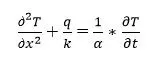
Considering steady state and integrating,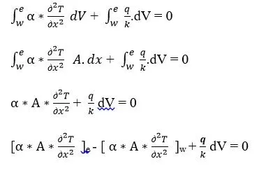
- Here, we use Gauss divergence theorem to convert from volume integral to surface integral in the partial derivative.
- In the above equation, 'α', 'A' and second degree derivative of temperature with respect to 'x' direction are to be known. Area is generally known. [(∂^2T)/(∂x^2)] are found using any of the differencing schemes. But 'α' value is dependent on temperature and it's value at each nodes are found using interpolation schemes.
- Interpolation profiles are then assumed in order to describe the variation of the concerned variable between cell centroids.
- The resulting equation is called the discretized or discretization equation. In this manner, the discretization equation expresses the conservation principle for the variable inside the control volume.
- Interpolation schemes:
Some of the common interpolation schemes are listed below.
1. Linear interpolation or central differencing:
By looking the figure below, the face values appearing in the convective flux can be computed as follows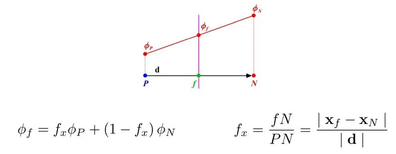
This type of interpolation scheme is known as linear interpolation or central differencing and it is second order accurate. However, it may generate oscillatory solutions (unbounded solutions).
2. Upwind differencing:
By looking the figure below, the face values appearing in the convective flux can be computed as follows,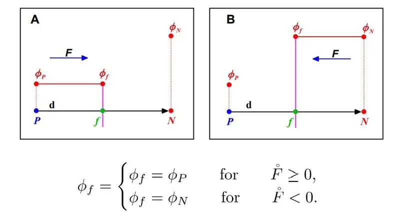
This type of interpolation scheme is known as upwind differencing and it is first order accurate. This scheme is bounded (non-oscillatory) and diffusive.
3. Second order upwind differencing (SOU) or linear upwind differencing (LUD) or Beam-Warming (BW)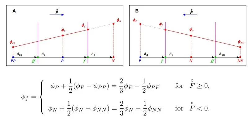
This type of interpolation scheme is known as second order upwind differencing (SOU), linear upwind differencing (LUD) or Beam-Warming (BW), and it is second order accurate. For highly convective flows or in the presence of strong gradients, this scheme is oscillatory (unbounded).
4. QUICK (Quadratic Upstream Interpolation for Convective Kinematics) - It is a higher-order differencing scheme that considers a three-point upstream weighted quadratic interpolation for the cell face values.
- In order to find the cell face value a quadratic function passing through two bracketing or surrounding nodes and one node on the upstream side must be used.
- In central differencing scheme and second order upwind scheme the first order derivative is included and the second order derivative is ignored. These schemes are therefore considered second order accurate where as QUICK does take the second order derivative into account, but ignores the third order derivative hence this is considered third order accurate.
- This scheme is used to solve convection–diffusion equations using second order central difference for the diffusion term and for the convection term the scheme is third order accurate in space and first order accurate in time. QUICK is most appropriate for steady flow or quasi-steady highly convective elliptic flow.
-
For the one-dimensional domain shown in the figure the Φ value at a control volume face is approximated using three-point quadratic function passing through the two bracketing or surrounding nodes and one other node on upstream side. In the figure, in order to calculate the value of the property at the face, we should have three nodes i.e. two bracketing or surrounding nodes and one upstream node.
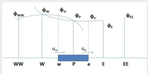
-
- Φw when uw > 0 and ue > 0 a quadratic fit through WW, W and P is used,
- Φe when uw > 0 and ue > 0 a quadratic fit through W, P and E is used,
- Φw when uw < 0 and ue < 0 values of W, P and E are used,
- Φe when uw < 0 and ue < 0 values of P, E and EE are used.
Let the two bracketing nodes be i and i − 1 and upstream node i – 2 then for a uniform grid the value of φ at the cell face between the three nodes is given by:

Flux limiters:
- To prevent oscillations in the SOU, we add a gradient or slope limiter function ψ(r) .
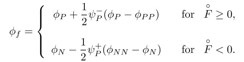
When the limiter detects strong gradients or changes in slope, it switches locally to low resolution (upwind).
• The concept of the limiter function ψ(r) is based on monitoring the ratio of successive gradients, e.g.,
- By adding a well designed limiter function ψ(r), we get a high resolution (second order accurate), and bounded scheme. This is a TVD scheme (Total Variation Dimensions scheme).
- A TVD scheme, is a second order accurate scheme that does not create new local undershoots and/or
overshoots in the solution or amplify existing extremes (high resolution). - The choice of the limiter function ψ(r) dictates the order of the scheme and its boundedness.
- The drawback of the limiters is that they reduce the accuracy of the scheme locally to first order, when r<=0 (sharp gradient, opposite slopes). However, this is justify when it serves to suppress oscillations.
- The various limiters have different switching characteristics and are selected according to the particular
problem and solution scheme. No particular limiter has been found to work well for all problems, and a
particular choice is usually made on a trial and error basis. - Some flux limiter functions are minmod,vanleer,superbee,Koren and CHARM
REFERENCES:
https://www.cfd-online.com/Wiki/Finite_volume
http://scholarpedia.org/article/Finite_volume_method
https://www.math.uci.edu/~chenlong/226/FVM.pdf
https://mathworld.wolfram.com/FiniteVolumeMethod.html
http://www.wolfdynamics.com/wiki/fvm_crash_intro.pdf
https://www.cfd-online.com/Forums/fluent/39028-difference-between-fem-fdm-fvm.html
http://www.nitttrc.edu.in/nptel/courses/video/112107079/lec29.pdf