Week 2 - Flow over a Cylinder.
AIM:
To simulate the flow over a cylinder and explain the phenomenon of Karman vortex street.
OBJECTIVE:
- To simulate the flow with the steady and unsteady case and calculate the Strouhal Number for Re= 100.
- To calculate the coefficient of drag and lift over a cylinder by setting the Reynolds number to 10,100,1000,10000 & 100000.
- To discuss the effect of Reynolds number on the coefficient of drag.
- To plot of the coefficient of drag and lift.
- Plots to show vortex shedding behind the cylinder.
Phenomenon of Karman vortex street:
In spite of extensive experimental and numerical studies almost over a century, flow around a circular cylinder still remains a challenging problem in fluid mechanics, where intensive investigations are continued even today to understand the complex unsteady dynamics of the cylinder wake flow. Cross-flow normal to the axis of a stationary circular cylinder and the associated problems of heat and mass transport are encountered in a wide variety of engineering applications. Both experimental measurements and numerical computations have confirmed the onset of instability of the wake flow behind a cylinder beyond a critical Reynolds number, leading finally to a kind of periodic flow identified by definite frequencies, well-known in the literature as the Von Karman vortex street.
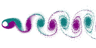
In fluid dynamics, a Kármán vortex street (or a von Kármán vortex street) is a repeating pattern of swirling vortices, caused by a process known as vortex shedding, which is responsible for the unsteady separation of flow of a fluid around blunt bodies.
A vortex street will form only at a certain range of flow velocities, specified by a range of Reynolds numbers (Re), typically above a limiting Re value of about 90. The (global) Reynolds number for a flow is a measure of the ratio of inertial to viscous forces in the flow of a fluid around a body or in a channel, and may be defined as a nondimensional parameter of the global speed of the whole fluid flow:

where:

 like the body speed relative to the fluid at rest, or an inviscid flow speed, computed through the Bernoulli equation), which is the original global flow parameter, i.e. the target to be non-dimensionalised.
 = a characteristic length parameter of the body or channel
 = the free stream kinematic viscosity parameter of the fluid, which in turn is the ratio:

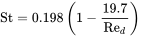

- f = vortex shedding frequency.
- d = diameter of the cylinder
- U = flow velocity.
Practical applications:
These are observed all over nature, e.g. wind flowing around mountains and islands; and play an important role in many engineering design problems. This is present any number of flow applications - ranging from cars passing through air to wind blowing across a smoke stack - where the air is not allowed to smoothly come back together after the obstruction.
They are of particular concern when the vortices are being generated at or near the natural frequency of the obstructions, as they can induce oscillations - leading to unwanted noise and vibration, and potentially structural failure.
1. Geometry:
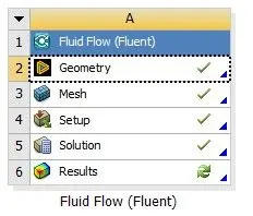
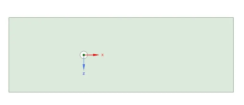
First step is to create geometry. Double click on the geometry and sketch the geometry as per requested in the question.
2. Meshing:
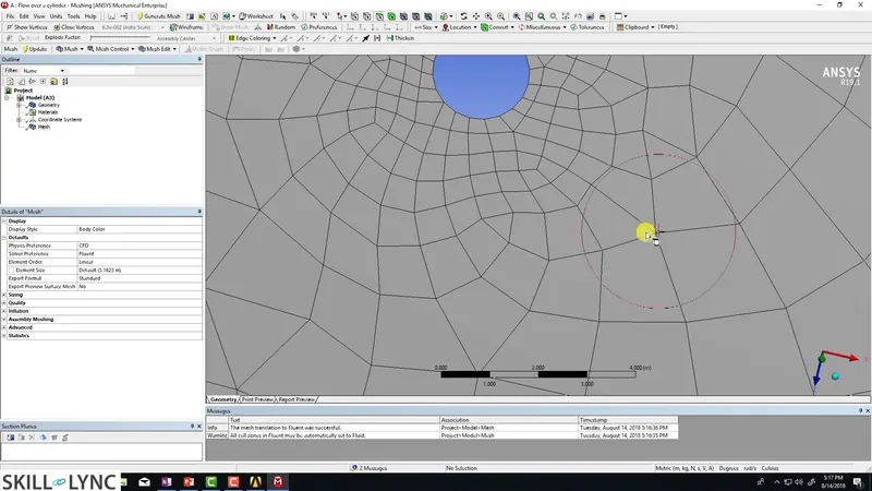
The second step is meshing. By clicking the mesh, it shows the default quadrilateral mesh with default size.
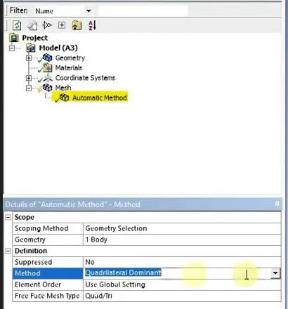
By clicking automatic method in mesh, the default values gets displayed. Change the quadrilateral dominant to triangular for finer mesh.
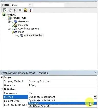
Now click generate mesh. The pink color in the mesh represents that the mesh is obselete. Then the mesh changes from quadrilateral to triangular. Then change the element sizt from default to 2 meters.
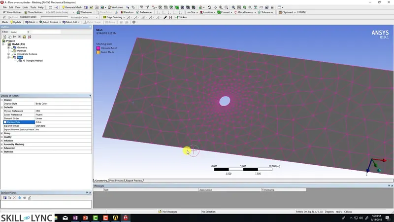
The triangular mesh is as shown in the figure. But the circle is polygonal in shape and not a perfect circle. In order to make perfect circle go to mesh. Right click it and select insert and sizing.
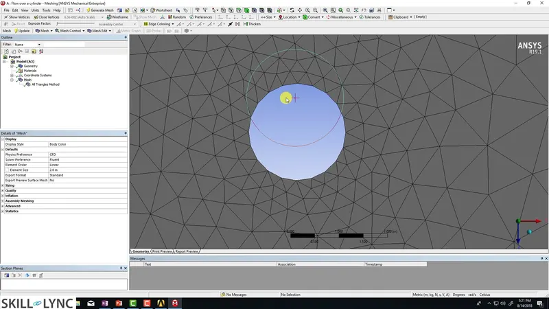
Sizing:
Select the edge which is needed to be sized and cliclk apply in the geometry. Now the geometry has become perfect circle so that there will not be disturbances during the flow.
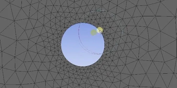
Inflation layer:
Now right click the mesh and select the inflation layer. Inflation layer helps us to create body fitted mesh.
In inflation option, select first layer thickness. In inflation thickness, select 0.005 (5 mm thick).
In the minimum layer option, select 2 for generating 2 layers. In the below case, 6 layers have been inserted.
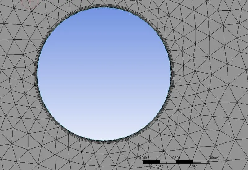
Now update the mesh.
Named selection (shortcut key 'N')
After that the boundary conditions are initialized by clicking the edge and pressing 'N' or right click it and select 'named selection'. Inlet(entry), Outlet(exit), wall(circular portion) and symmetry boundary condition (top and bottom layers).
3.Setup:
- Now update the setup as well after closing mesh.
- Now select 'Physics' and click on boundaries. Now click on check mesh and check then meshing properties and verify it.
- In 'Physics' option, select 'pressure based solver' and 'steady' condition.
- Now select 'viscous' and click 'laminar' option.
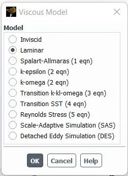
- Now select 'materials' and change the name, density and viscosity value.
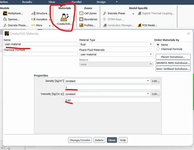
Now select 'boundary' and insert inlet velocity and other boundary condition parameters and click ok.
Selecting monitor point:
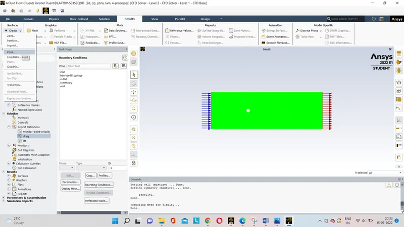
In order to take the reading of the particular parameter, at a particular point monitor point velocity has to be fixed in the geometry region. So for making moniter point, go to post processing and select 'create' ---> 'point' .
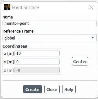
After that, a window will open where 'X' and 'Y' coordinates are entered for locating that particular point.
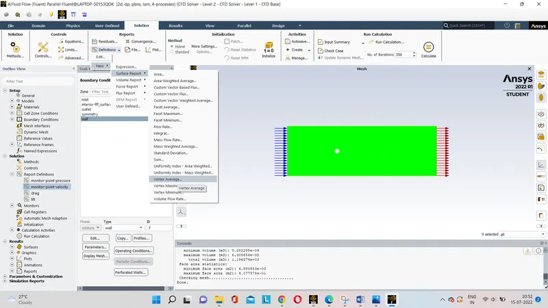
Now select Solution and click 'Defnition' ---> 'new' ---> 'Surface report' ---> 'Vertex average' and select the required parameter to be studied (eg: velocity, pressure) at the monitor point.
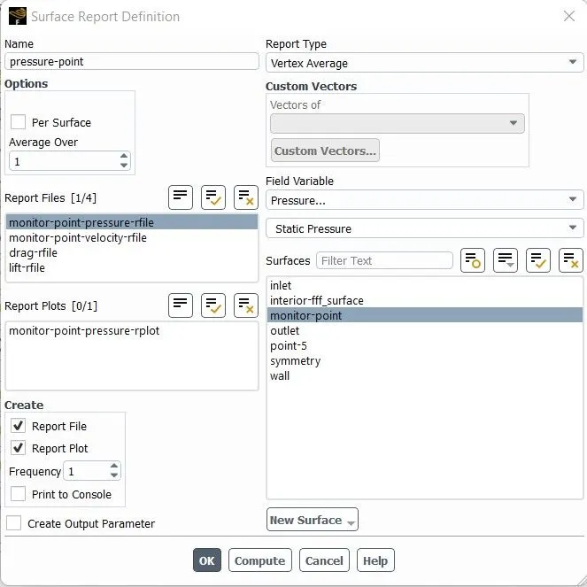
Now initialize the domain.
Contour plot:
For making contour plot, select post processing after making monitor point and initialization. Tick mark filled option and select all the parameters for making contour plot.
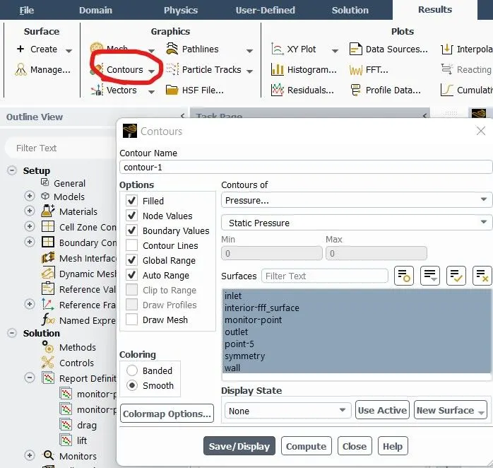
The contour of the required parameters such as 'pressure', 'velocity' is to be selected and save/Display and select compute.
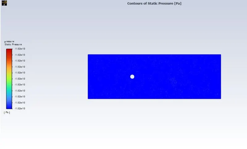
Pressure contour plot:
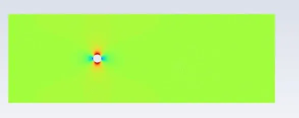
Velocity contour plot:
Residuals:
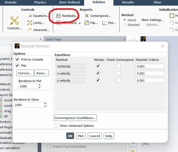
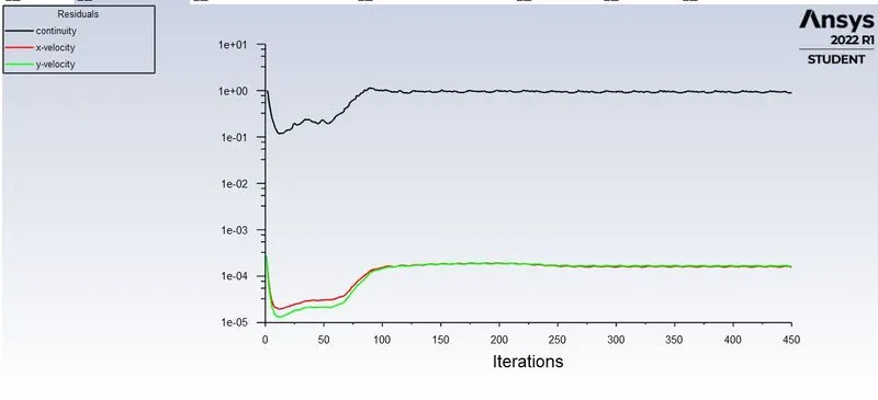
Now go to 'solution' and select 'residuals'. The residuals for continuity equation, 'x' velocity and 'y' velocity are determined.
Animations:
For animations, go to 'Solution' select 'create' ---> 'animations' in the activity toolbar.
The animation toolbar will appear. Select the parameter in which the animation has to be created and select the record after number of iteration the animation has to be displayed. Click ok.
Calculate:
Then click calculate for approx 350 iterations.
RESULTS:
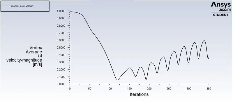
Velocity plot for Steady case for Reynolds number 100:
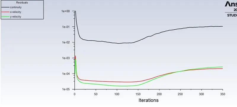
Residual plot for Steady case for Reynolds number 100:
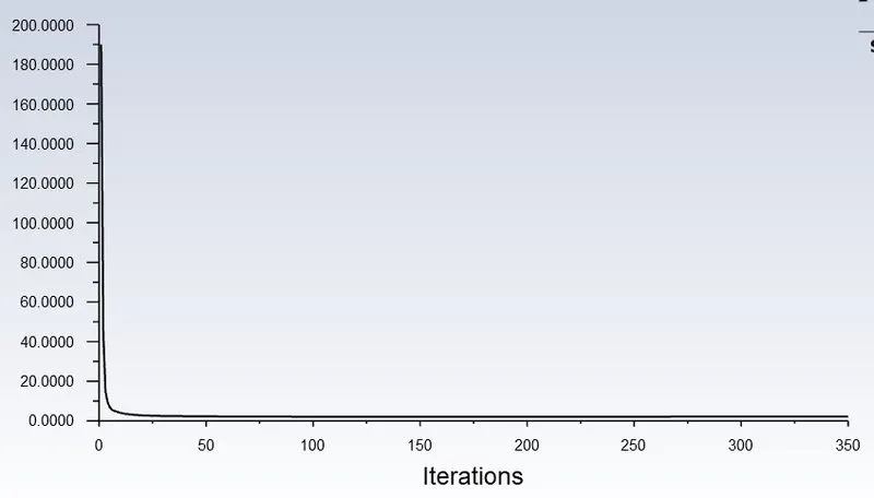
Co-efficient of drag plot for Steady case for Reynolds number 100:
Co-efficient of lift plot for Steady case for Reynolds number 100:
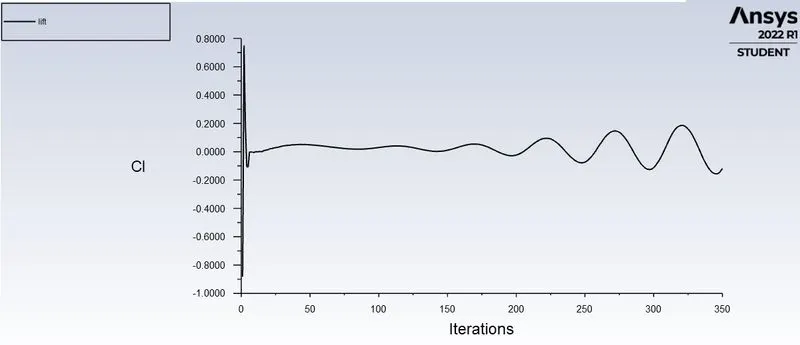
Velocity Contour plot for Steady case for Reynolds number 100:
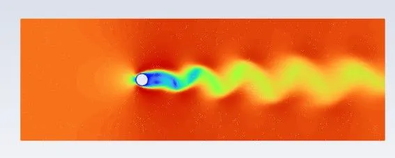
Pressure contour plot for Steady case for Reynolds number 100:
Transient case simulation (Re 100):
Velocity plot for unsteady case for Reynolds number 100:
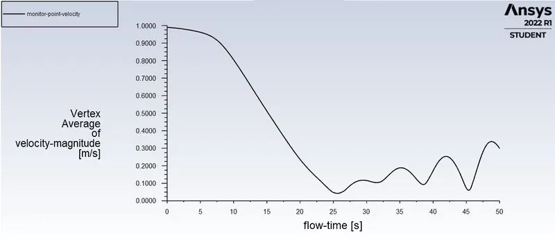
Pressure plot for unsteady case for Reynolds number 100:
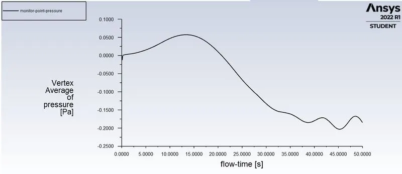
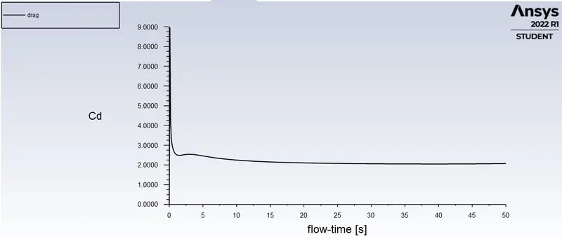
Drag plot for unsteady case for Reynolds number 100:
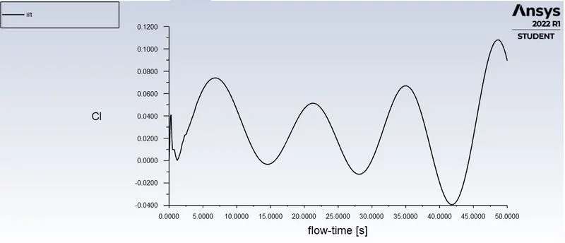
Lift plot for unsteady case for Reynolds number 100:
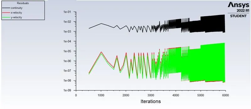
Residuals plot for unsteady case for Reynolds number 100:
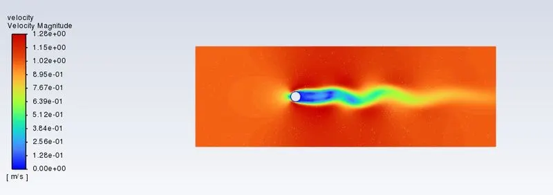
Velocity Contour plot for unsteady case for Reynolds number 100:
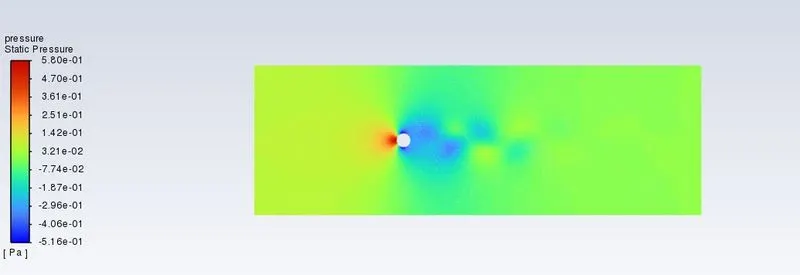
Static pressure contour plot for unsteady case for Reynolds number 100:
CASE 2:
Plots for Reynolds number 1000
Residuals plot for steady case - Reynolds number: 1000:
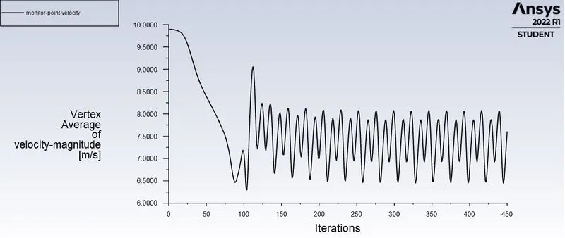
Velocity plot for steady case - Reynolds number: 1000:
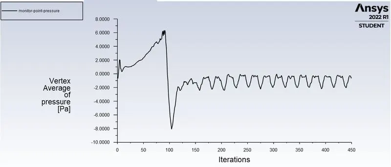
Pressure plot for steady case - Reynolds number: 1000:
Contour plot for steady case - Reynolds number: 1000:
Co-efficient of drag plot for steady case - Reynolds number: 1000:
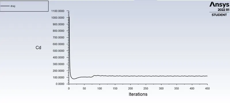
Co-efficient of lift plot for steady case - Reynolds number: 1000:
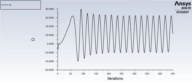
Plots for Reynolds number 10:
Co-efficient of drag plot for steady case - Reynolds number: 10:
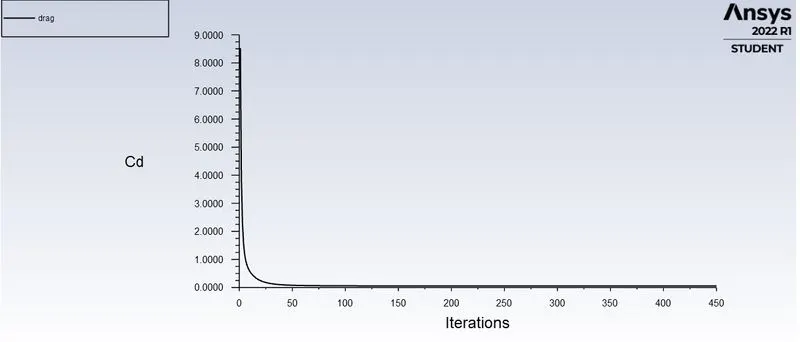
Co-efficient of lift plot for steady case - Reynolds number: 10:
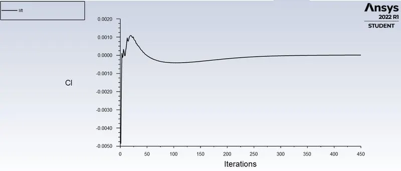
Plots for Reynolds number 10000:
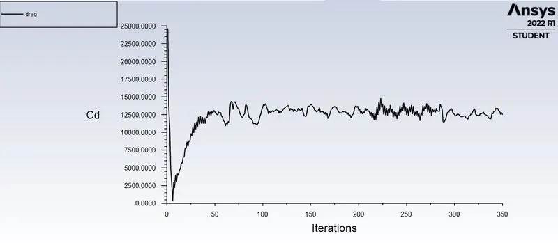
Co-efficient of drag plot for steady case - Reynolds number: 10000:
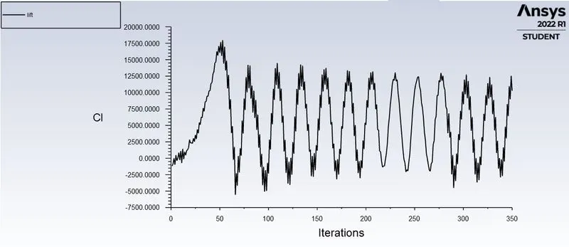
Co-efficient of lift plot for steady case - Reynolds number: 10000:
CONCLUSION:
Thus the plots with the different Reynold's number are simulated and made as per given in the question.
It can be concluded that the steady state plots can be more smoother than the unsteady state.