Week 3 - Solving second order ODEs

AIM:

To write a program that solves the ODE which represents the equation of motion of a simple pendulum with damping.

GOVERNING EQUATION:

d²θ/dt² + (c/m)*(dθ/dt) + (g/l)*sin θ

where,
θ = angular displacement (degrees)

t = time (seconds)

c = damping coefficient

m = mass (kilogram)

g = acceleration due to gravity(m/s²)

l = length of the string (meters)

Here,

θ = θ₁

(d θ/dt) = (d θ₁/dt) = θ₂ …………….(2)

(d² θ/dt) = (d² θ ₁/dt²) = d/dt(θ₂)

From equation (1),

d²θ/dt² + (c/m)*(dθ/dt) + (g/l)*sin θ = 0

therefore, d²θ₁/dt² + (c/m)*(dθ₁/dt) + (g/l)*sin θ₁ = 0

dθ₂/dt + (c/m) θ₂ + (g/l)*sin θ₁ = 0

dθ₂/dt = -(c/m) θ₂ - (g/l)*sin θ₁ …………….(3)

OBJECTIVES OF THE PROJECT:

1. To write a code that solves the ODE of the simple pendulum with damping.
2. To obtain a graph which shows the Displacement vs Time and Velocity vs Time diagram.
3. To make the animation of the motion of the simple pendulum with the following assigned values.
   
   L=1 metre,

m=1 kg,

c=0.05.

g=9.81 m/s2.

4. To Simulate the motion between 0-20 sec, for angular displacement=0,angular velocity=3 rad/sec at time t=0.

BODY OF CONTENT:

close all
clear all
clc
 
c = 0.05;
g = 9.81;
l = 1;
m = 1;
 
% initial conditions
theta_0 = [0;3];
 
% time points
t_span = linspace(0,20,100);
 
% solve ODE
[t, results] = ode45(@(t, theta) ode_func(t, theta, c,g,l,m),t_span, theta_0);
 
plot(t,results(:,1))
hold on
plot(t,results(:,2))
xlabel('time')
ylabel('plot')

Explanation:

The initial values c,g,l,m is assigned as given in the question. The initial conditions ‘theta_0’ is assigned with 2 column vector of initial angular displacement and initial angular velocity.

Then the time span value is given with range of 0 to 20 seconds with the help of ‘linspace’ command with 100 values in between.

Then the ODE function is called. ‘ode45’ is an inbuilt solver in matlab. In ‘ode45’, the main inputs are time(t) and angular displacement(θ) where the time is an independent variable and angular displacement is dependent variable.

‘ode_func’ consists of inputs as t,theta,c,g,l,m. Then it consists of initial conditions. Here ‘ode_func‘ is written in a separate matlab sub program which is explained later.

Then the graph is plotted between independent variable time and dependent variable angular displacement by using ‘plot’ command. Here the plot command is represented as
plot(t,results(:,1)) which represents the plot between time variable and results of the first column vector which is obtained from ‘ode45’ inbuilt solver.

Then ‘hold on’ command is used so that the plot would not disappear. Then plotting is done between independent variable ‘time’ and dependent variable velocity similar to above.
plot(t,results(:,2)). which represents the plot between time variable and results of the second column vector which is obtained from ‘ode45’ inbuilt solver.

Then ‘xlabel’ and ‘ylabel’ input is given which is to be displayed in ‘x axis’ and ‘y axis’.

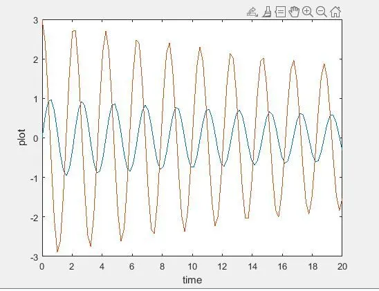
Here blue line represents the angular displacement and red line represents the angular velocity.

Supplementary program:

function [dtheta_dt] = ode_func(t,theta,c,g,l,m)

theta1 = theta(1)
theta2 = theta(2)
dtheta1_dt = theta2;
dtheta2_dt = -(c/m)*theta2 - (g/l)*sin(theta1);
dtheta_dt = [dtheta1_dt; dtheta2_dt];
end

Here as per the derivation θ₁ and θ₂ are given as theta(1) and theta(2).

As per first ODE (dθ₁/dt) = θ₂

As per second ODE (dθ₂/dt) = (-c/m) θ₂ – (g*sind(θ₁))/L

These ODE1 and ODE2 has been combined into an array to provide 2 coloumns where one column represents the angular displacements and the other represents the angular velocity.

This supplementary program defines the ‘ode_func’ in the main program which gives the final graph.

Program to create animation of motion of Simple Pendulum:

close all
clear all
clc

c = 0.05;
g = 9.81;
l = 1;
m = 1;

% initial conditions
theta_0 = [0;3];

% time points
t_span = linspace(0,20,100);

% solve ODE
[t, results] = ode45(@(t, theta) ode_func(t, theta, c,g,l,m),t_span, theta_0);

plot(t,results(:,1))
hold on
plot(t,results(:,2))
xlabel('time')
ylabel('plot')

disp = results(:,1)
ct = 1;
for i = 1:length(t_span)
    x0 = 0
    y0 = 0
    
    x1 = l*sind(disp(i));
    y1 = -l*cosd(disp(i));
    	
    % plotting
    plot([-0.05 0.05],[0 0],'linewidth',5,'color','b')
    hold on
    plot([x0 x1],[y0 y1],'linewidth',3,'color','r')
    hold on
    axis([-.1 .1 -2 0])
    plot(x1,y1,'marker','O','markersize',20,'markerfacecolor','g')
    hold on
    pause(0.05)
    hold off
    M(ct) = getframe(gcf);
    ct=ct+1;
end
 
 
movie(M)
videofile = VideoWriter('simple_pendulum_motion.avi','Uncompressed AVI');
open(videofile)
writeVideo(videofile,M)
close(videofile)

Explanation:

After writing code for ODE for simple pendulum equation, the animation for the motion of simple pendulum is to be obtained. To get that ‘for’ loop command is used. The results of first column in the array which are the values of angular displacement is assigned as ‘disp’ variable. The counter value is given as ‘ct = 1’

Then the ‘i’ value in ‘for’ loop is counted from 1 to length of ‘t_span’ which is 20 seconds. Then the position of the angular displacement of the simple pendulum is assigned for each time value as given below.

x0 = 0

y0 = 0

x1 = l*sind(disp(i));

y1 = -l*cosd(disp(i));

Then plotting is done using ‘plot’ command of the angular positions of the given values for respective time period for the string of the pendulum.

‘Hold on’ command is used to hold the plotting position without disappearing when the next command in the program is executed.

Then the ball of the simple pendulum is obtained using ‘marker’ command.

‘Marker’ command syntax:

plot(position of the marker,’marker’,’symbol of the marker’,’markersize’,value of the marker size,'markerfacecolor',’desired color’)

Then the position of the pendulum is paused for 0.05 seconds.

Then ‘hold off’ command is given, otherwise the angular position of the pendulum will not fade off and the motion of the pendulum will not be clear.

Then counter value is increased by 1 value, which the next iteration will be proceeded in the ‘for’ loop.

To make this collection of the frames like a movie, ‘movie(M)’ command is used. Then this video file is saved in the ‘VideoWriter’ command.

Errors faced:

1. In ‘for’ loop, while assigning the position of the string for each time period, the length is assigned as
   x1 = l*sind(disp) and y1 = -l*cosd(disp) and ‘disp’ is assigned as
   disp = results(:,1) which is an array of elements. But ‘x1’ and ‘y1’ should be an integer of single term. So the command window displayed the error mentioned as ‘Dimentions of arrays being concatenated are not consistent’. It is noticed and the error is corrected.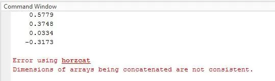
   
   
   
   
   
2. The values for ‘x1’ and ‘x2’ in the ‘for’ loop is assigned as
   x1 = l*cosd(disp(i)) and y1 = -l*sind(disp(i))
   Thus the simple pendulum animation instead of oscillating from 3^rd and 4^th quadrant, it oscillated in the 1^st and 4^th It has been noticed and the allotment values for ‘x1’ and ‘y1’ are corrected to
   x1 = l*sind(disp) and y1 = -l*cosd(disp)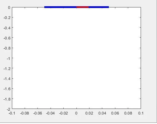
   
   

RESULTS AND CONCLUSION:

Thus the code that solves the ODE of the simple pendulum with damping using matlab is obtained and in the results, it has been found that the displacement and velocity graph amplitude decreases for each cycle as the damping co-efficient increases. As the damping co-efficient value is very high, the motion is brought to rest in short span of time and the animation for the motion of the simple pendulum is made using matlab. The link for the animation is uploaded in google drive and also in the following link below

https://drive.google.com/file/d/1KN2az58_23US7jUCe4-IAlce5vWtB_MP/view?usp=sharing