Week 5.1 - Mid term project - Solving the steady and unsteady 2D heat conduction problem
AIM:
- To solve the 2D heat conduction equation by using the point iterative techniques for the boundary conditions for the problem are as follows;
Top Boundary = 600 K
Bottom Boundary = 900 K
Left Boundary = 400 K
Right Boundary = 800 K
By implementing the following methods to solve the implicit equations.
1. Jacobi
2. Gauss-seidel
3. Successive over-relaxation
absolute error criteria is 1e-4
- To write code for both implicit and explicit schemes for the Transient Analysis only.
- To write a code for steady state 2D heat conduction equation for 3 iterative methods.
- To make a detailed explanation for the results and plots obtained.
GOVERNING EQUATION:
Steady state 2-D Heat conduction equation:
(ꝺ2T/ ꝺx2) + (ꝺ2T/ ꝺy2) = 0
By integrating and solving we get,
Tp = ((TL + TR)/(dx2) + (TT + TB)/(dy2))/K
where,
Tp= Temperature at the required grid point
TL= Adjacent temperature to the left of the grid point
TR= Adjacent temperature to the right of the grid point
TT= Adjacent temperature to the top of the grid point
TB= Adjacent temperature to the bottom of the grid point
K =2*(dx^2+dy^2)/(dx^2*dy^2)
Temperature for Successive Over Relaxation iterative method:
T(i,j) = (1-w)*Told + w*T_gs
T(i,j)= Temperature at the specific i,j point.
Told = Temperature at previous step
T_gs= Temperature in the Gauss Seidal iterative method
w = Constant
Unsteady Transient State Solution:
Explicit scheme:
((ꝺ2T/ ꝺx2) + (ꝺ2T/ ꝺy2) )*α = ꝺT/ ꝺt
By integrating and solving we get,
Tpn+1 = Tpn + K1 * (TL - 2*Tp + TR)n + K2 * (TT - 2*Tp + TB)n
where,
The equation on the left hand side is for (n+1)th time step and the equation on the right hand side is for nth time step.
Tp= Temperature at the required grid point
TL= Adjacent temperature to the left of the grid point
TR= Adjacent temperature to the right of the grid point
TT= Adjacent temperature to the top of the grid point
TB= Adjacent temperature to the bottom of the grid point
K1 = α*(dt/(dx^2)) & K2 = α*(dt/(dy^2))
where α = Thermal diffusivity
CFL1 = K1 & CFL2 = K2
where
CFL1 + CFL2 <= 0.5 (Stability condition)
Unsteady Transient State Solution:
Implicit scheme:
Tpn+1 = (term1*Tpn )+ (term2 * (TL + TR)n+1 ) + term3 * (TT + TB)n+1
where
term1 = 1/(1+2*K1+2*K2)
term2 = K1*term1
term3 = K2*term1
BODY OF CONTENT:
Theory:
Linear equation systems are linked to many engineering and scientific topics, as well as quantitative industry, statistics, and economic problems. It is possible and easy to solve a large number of symmetric, linear algebraic equations after the invention of computers. The solution of a very large set of simultaneous equations by numerical methods in time is an important factor in the practical application of the results. If the equations are solved in considerable time, we can increase productivity significantly.
We have mainly two numerical methods: the direct method and the iterative method for solving linear equation systems. For a big set of linear equations, particularly for sparse and structured coefficient equations, the iterative methods are preferable as they are largely unaffected by round-off errors. The well known classical iterative methods are the Jacobian and Gauss-Seidel methods. Here, we are going to discuss the Jacobi or Jacobi Method.
Jacobian Iteration method:
Matrices in the form of "AX=b" can easily represent a large linear system, where "A" represents a square matrix containing the ordered coefficients of our system of linear equations, "X" contains all of our various variables, and "B" represents the constants equal to each linear equation. For our unknown x-values, we wish to solve, and we can do so by using the Jacobian Method. As discussed, we can summarize the Jacobi Iterative Method with the equation "AX=B." The "a" variables indicate the elements of the "A" coefficient matrix, the "x" variables give us the unknown X-values which we are solving for, and the constants of each equation are represented by "b".
Now, AX=B is a system of linear equations, where
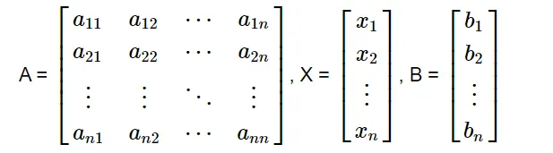
Suppose that none of the diagonal entries are zero without loss of generality; otherwise, swap them in rows, and the matrix A can be broken down as,
A=(D+U+L) ,
where D is the Diagonal matrix of A, U denotes the elements above the diagonal of matrix A, and L denotes the elements below the diagonal of matrix A
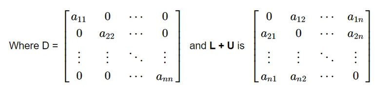
The solution can be obtained iteratively via using the following relation:

Where Xk and X(k+1) are kth and (k+1)th iteration of X. The elements of X(k+1) can be calculated by using element based formula that is given below:

Therefore, after placing the previous iterative value of X in the equation above, the new X value is determined until the necessary precision is achieved. The vital point is that the method should converge in order to find a solution. The sufficient but not possible condition for the method to converge is that the matrix should be strictly diagonally dominant. The Jacobi Method is also known as the simultaneous displacement method.
Gauss-Seidel and Jacobi Methods
The difference between Gauss-Seidel and Jacobi methods is that, Gauss Jacobi method takes the values obtained from the previous step, while the Gauss–Seidel method always uses the new version values in the iterative procedures. The reason why the Gauss-Seidel method is commonly referred to as the successive displacement method is that the second unknown is calculated by the first unknown in the current iteration, the third unknown is calculated from the 1st and 2nd unknown, etc.
Successive Over Relaxation method:
In numerical linear algebra, the method of successive over-relaxation (SOR) is a variant of the Gauss–Seidel method for solving a linear system of equations, resulting in faster convergence. A similar method can be used for any slowly converging iterative process.
The successive overrelaxation method (SOR) is a method of solving a linear system of equations  derived by extrapolating the Gauss-Seidel method. This extrapolation takes the form of a weighted average between the previous iterate and the computed Gauss-Seidel iterate successively for each component,
 |
where  denotes a Gauss-Seidel iterate and
  is the extrapolation factor. The idea is to choose a value for that will accelerate the rate of convergence of the iterates to the solution.
If  , the SOR method simplifies to the Gauss-Seidel method. A theorem due to Kahan (1958) shows that SOR fails to converge if is outside the interval
  .
.
In general, it is not possible to compute in advance the value of that will maximize the rate of convergence of SOR. Frequently, some heuristic estimate is used, such as  where
where  is the mesh spacing of the discretization of the underlying physical domain.
MATLAB CODE:
Matlab code for Steady 2-Dimensional heat conduction equation using 3 iterative methods:
close all
clear all
clc

% Code for 2nd order 1-d pde
% d^2u/dx^2 +  d^2u/dy^2

%inputs
nx = 10;
ny = 10;

%Boundary conditions
T_top = 600;
T_bot = 900;
T_left = 400;
T_right = 800;

%Initial Temperature assumption
T = ones(nx,ny);

T(1,:) = T_top;
T(end,:) = T_bot;
T(:,1) = T_left;
T(:,end) = T_right;

% number of grid points
x = linspace(0,1,nx);
y = linspace(0,1,ny);

%Grid spacing
dx = x(2)-x(1);
dy = y(2) - y(1);

%Constant 'K'
k = 2*(dx^2+dy^2)/(dx^2*dy^2);

%Corner refinement
T(1,1) = (T_top+T_left)/2;
T(1,end) = (T_top+T_right)/2;
T(end,1) = (T_left+T_bot)/2;
T(end,end) = (T_bot+T_right)/2;

%error
error = 10;

%tolerance
tol = 1e-4;

%Initialization
Told = T;
Tinitial = T;

%Gauss Jacobi

iter_num_jac = 0
while(error>tol);

    for i = 2:nx-1
        for j = 2:ny-1
            T(i,j) = ((Told(i-1,j)+Told(i+1,j))/(dx^2)+(Told(i,j-1)+Told(i,j+1))/(dy^2))/k;
        end
    end
    error = max(max(abs(T-Told)));
    Told = T;

    figure(1)
    iter_num_jac = iter_num_jac+1;
    contourf(T,'ShowText','ON');
    title(sprintf('Steady state Jacobi 1D HCE iteration number = %d', iter_num_jac));
    pause(0.001);
    set(gca,'YDIR','reverse');

end

colorbar


% Gauss Seidal method

%Reinitializing
T = Tinitial;
Told = T;
error = 100;

iter_num_gs = 0
while(error>tol);


    for i = 2:nx-1
        for j = 2:ny-1
            T(i,j) = ((T(i-1,j)+T(i+1,j))/(dx^2)+(T(i,j-1)+T(i,j+1))/(dy^2))/k;
        end
    end
    error = max(max(abs(T-Told)));
    Told = T;

    figure(2)
    iter_num_gs = iter_num_gs+1;
    contourf(T,'ShowText','ON');
    title(sprintf('Steady state Gauss Seidal 1D HCE iteration number = %d', iter_num_gs));
    pause(0.001);
    set(gca,'YDIR','reverse');

end
colorbar


%SOR method

%Reinitializing
T = Tinitial;
Told = T;
error = 100;
w = 1.3

iter_num_sor = 0
while(error>tol);


    for i = 2:nx-1
        for j = 2:ny-1
            T_gs(i,j) = ((T(i-1,j)+T(i+1,j))/(dx^2)+(T(i,j-1)+T(i,j+1))/(dy^2))/k;
            T(i,j) = (1-w).*Told(i,j)+w.*T_gs(i,j);
        end
    end
    error = max(max(abs(T-Told)));
    Told = T;

    figure(3)
    iter_num_sor = iter_num_sor+1;
    contourf(T,'ShowText','ON');
    title(sprintf('Steady state SOR 1D HCE iteration number = %d', iter_num_sor));
    pause(0.001);
    set(gca,'YDIR','reverse');

end
colorbar
Explanation:
- First, the initial input conditions are given. The number of grid points in 'x' and 'y' direction are given as input.
- Then the given boundary conditions at top,bottom,left and right are entered as given in question.
- The length of the domain is assumed to be 1 unit length and 1 unit height and they are divided into 'nx' & 'ny' number of grid points in 'x' and 'y' direction using 'linspace' command.
- Grid spacing is the difference between the adjacent grid points.
- At corners, the temperature is assumed to be the average of their adjacent points. Then the value of 'K' is entered as per given in the formula.
- Initial error is assumed to be 10(any value of positive integer is considered) and tolerance is entered as given in the question.
- Initial iteration number is entered to calculate total number of iterations required to get the final solution.
- When error is greater than tolerance, then the iterations has to be performed to converge to a accurate solution with acceptable tolerance. This is done using 'while' loop with condition of (error>tolerance). The iteration is repeated until this condition is satisfied. When this condition fails, the final optimal solution is obtained.
- Then the value of temperature at each grid points is calculated using the formula that is mentioned in the governing equation for 3 iterative methods separately using nested 'for' loop.
- After calculating the temperature values at each grid points in the domain, the error has to be checked which is the maximum difference of temperature values of current Temperature values and the old temperature values at respective points. It is done using the command 'error = max(max(abs(T-Told)))'.
[Here 'max' is used 2 times since the domain is 2-dimensional so that the maximum error value at 'entire surface area is calculated]. - Then, the present Temperature values is updated as 'Told' values which for the next iteration the old temperature values is taken from the result of the previous iteration.
- Then the iteration counter is increased to 1, to keep the values updated for number of iteration.
- Then, the diagram is plotted using 'contourf' command where the plots for each iteration is displayed with differentiated colors according the the respective values.
- Now the title is given using 'title' command where the title along with number of iterations is displayed in the heading using 'sprintf' command.
- The plot is paused for 0.001 second before the next iteration plot appears using 'pause' command.
- Now the values obtained is displayed in the plot in a tilted manner since the 'contourf' takes the last value data and displays first. So the plot has to be tilted. This is done using ''set(gca,'YDIR','reverse')'' command.
- Finally, 'colorbar' shows the values of the colored portion range in the plot at right side of the graph. (similar to legend).
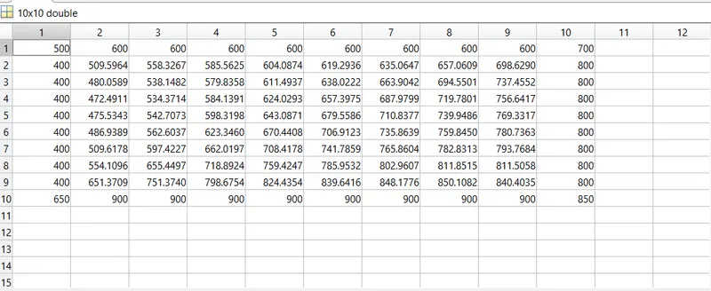
The above graph shows the final converged data for 2-D heat conduction problem. These values are represented in the graph as shown in the results below.
RESULTS:
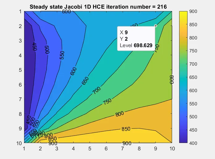
Plot for Steady state 2-Dimensional heat conduction equation using Gauss Jacobi iterative method:
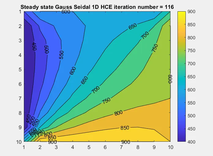
Plot for Steady state 2-Dimensional heat conduction equation using Gauss Seidal iterative method:
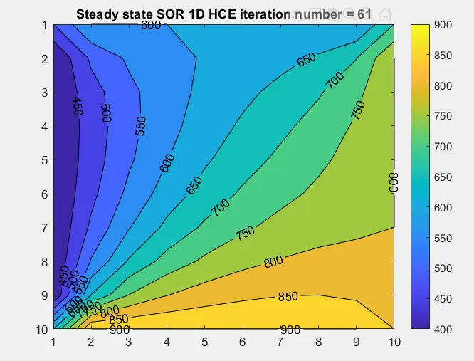
Plot for Steady state 2-Dimensional heat conduction equation using Successive Over Relaxation (SOR) iterative method:
OBSERVATION AND DISCUSSION FROM THE RESULT:
- It is observed from the result that SOR(Successive Over Relaxation) method takes least number of iterations and Gauss Jacobi method takes more number of iterations to converge to a final solution and Gauss Seidal method takes number of iterations inbetween 'Gauss Jacobi' and 'SOR'.
- The SOR method converges approximately 4 times faster than the Jacobi and Gauss Seidal method converges approximately 2 times faster than the Jacobi.
- From the iteration it has been concluded that in SOR method as the 'w' value(constant) decreases, the convergence rate is very low or it takes more number of iterations to get the optimal final solution compared to the Seidal and Jacobi also.
For example, for w=0.1, it took 1750 iteration to reach final solution.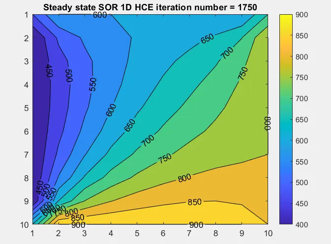
If the 'w' value is very high, the solution becomes unstable and takes more number of iterations and expected plot is not obtained. So it is necessary to give the 'w' value inbetween (1-1.5) to converge at faster rate.
For example, for w = 2.5, it took 1725 number of iteration and the expected result also not obtained.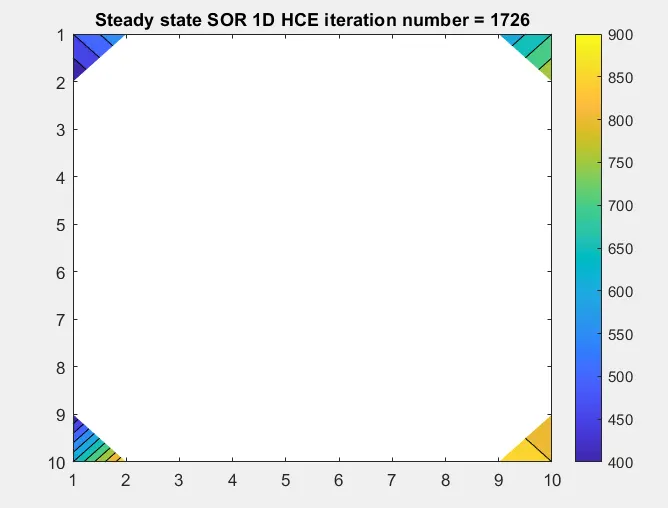
Matlab code for Transient 2-Dimensional heat conduction equation using explicit scheme:
clear all
close all
clc

% Transient state heat conduction equation for Explicit scheme

%Inputs
nx = 10;
ny=nx;

%Boundary conditions
T_top = 600;
T_bot = 900;
T_left = 400;
T_right = 800;

%Initial Temperature assumption
T = ones(nx,ny);

T(1,:) = T_top;
T(end,:) = T_bot;
T(:,1) = T_left;
T(:,end) = T_right;

% number of grid points
x = linspace(0,1,nx);
y = linspace(0,1,ny);

%Grid spacing
dx = x(2)-x(1);
dy = y(2) - y(1);

%Thermal diffusivity
alpha = 1.5;

%Time step assumption
dt = 1e-1;

%Constant 'K'
k1 = alpha*dt/(dx^2);
k2 = alpha*dt/(dy^2);

%Corner refinement
T(1,1) = (T_top+T_left)/2;
T(1,end) = (T_top+T_right)/2;
T(end,1) = (T_left+T_bot)/2;
T(end,end) = (T_bot+T_right)/2;

%error
error = 10;

%tolerance
tol = 1e-4;

Told = T;
Tinitial = T;

cfl = k1+k2;


for q = 1:1400


    for i = 2:nx-1
        for j = 2:ny-1
            T(i,j) = (Told(i,j) + k1*(Told(i-1,j)-2*Told(i,j)+Told(i+1,j))+k2*(Told(i,j+1)-2*Told(i,j)+Told(i,j-1)));
        end
    end

    Told = T;

    figure(1)
    contourf(T,'ShowText','ON');
    colorbar

    title(sprintf('Transient Explicit 2D HCE '));
    pause(0.001);
    set(gca,'YDIR','reverse');

end
Explanation:
- The initial condition, inputs, boundary conditions, number of grid points, grid spacing is similar for explicit also like previous one.
- Here thermal diffusivity is given as 1.5 (assumed) and the time step is entered as 1e-3 which are the essential parameters for the transient state problems.
- The constant 'k1' and 'k2' are required in the formula obtained from the governing equation to find the temperature values. The 'k1' and 'k2' represents the CFL numbers. It is noted that CFL <= 0.5.
- Here, the 'while' loop is not necessary since it takes the 'Told' values and the counter is not required since the number of time steps is assumed to be 1400.
- Then the iteration is done by using the formula obtained from the governing equation using nested 'for' loop.
- Then the obtained temperature values is updated as 'Told' for next iteration.
- Finally figure is plotted using 'contourf' command.
RESULTS:
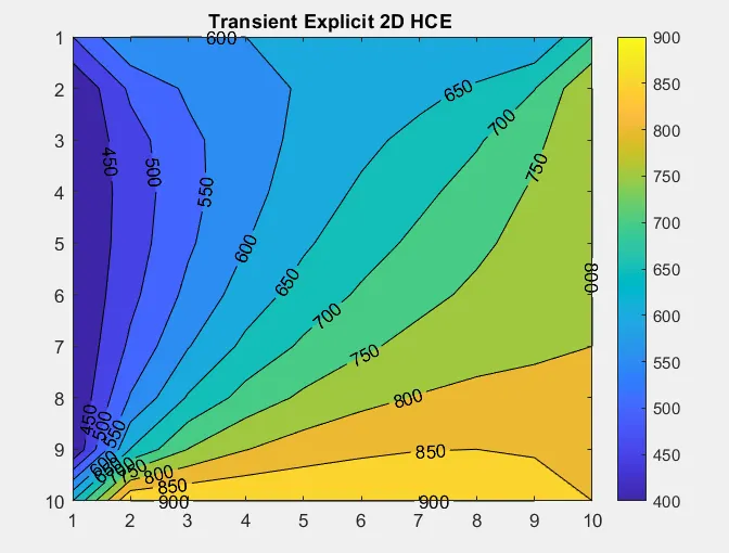
Plot for Transient state 2-Dimensional heat conduction equation using Explicit scheme:
OBSERVATION AND DISCUSSION FROM THE RESULT:
- It is observed from the result that when the time step value increases, the 'k1' value and 'k2' value increases since K1 = α*(dt/(dx^2)) and K2 = α*(dt/(dy^2)) which represents the CFL numbers (k1=CFL1 & k2=CFL2). But for stability condition, the total CFL number (CFL = CFL1 + CFL2) should be less than or equal to 0.5.
- So either by increasing 'α' value or time step value or by decreasing the grid spacing value, in such cases there is probablity that CFL crosses 0.5 which the result leads to instability.
- So lower time step value is chosen.
For example, In case of 1e-1 time step value, the result leads to instability and the plot obtained is as shown below.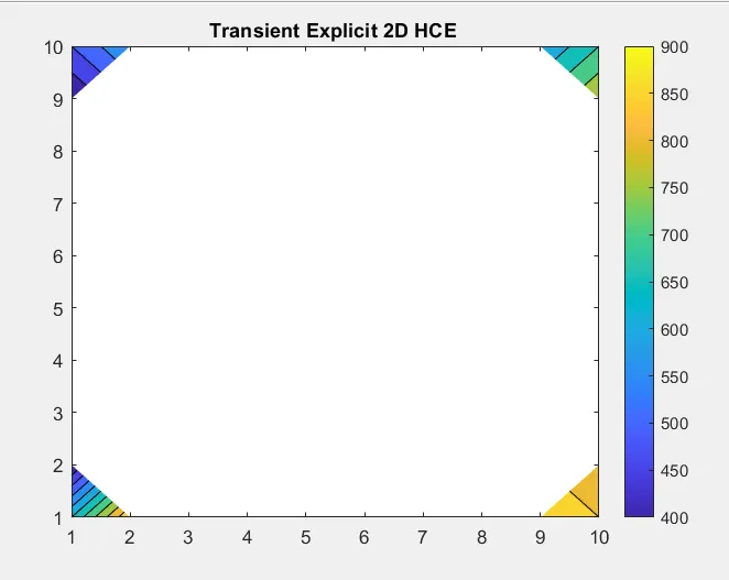
- This type of unstability plot is obtained when thermal diffusivity value is too high also.
Matlab code for Transient 2-Dimensional heat conduction equation using implicit scheme:
clear all
close all
clc

% Transient state heat conduction equation for Implicit scheme

%Inputs
nx = 10;
ny=nx;

%Boundary conditions
T_top = 600;
T_bot = 900;
T_left = 400;
T_right = 800;

T = ones(nx,ny);

T(1,:) = T_top;
T(end,:) = T_bot;
T(:,1) = T_left;
T(:,end) = T_right;

% number of grid points
x = linspace(0,1,nx);
y = linspace(0,1,ny);

%Grid spacing
dx = x(2)-x(1);
dy = y(2) - y(1);

%Thermal diffusivity
alpha = 1.5;

%Time step
dt = 1e-2;

%Constant 'K'
k1 = alpha*dt/(dx^2);
k2 = alpha*dt/(dy^2);

%Corner refinement
T(1,1) = (T_top+T_left)/2;
T(1,end) = (T_top+T_right)/2;
T(end,1) = (T_left+T_bot)/2;
T(end,end) = (T_bot+T_right)/2;

%error
error = 10;

%tolerance
tol = 1e-4;

Told = T;
Tprev = T;
Tinitial = T;

cfl = k1+k2

term1 = 1/(1+2*k1+2*k2);
term2 = k1*term1;
term3 = k2*term1;

%number of time steps
nt = 1400

iter_num = 0

%1-D HCE for Implicit scheme by Gauss Seidal

for q = 1:nt

    %Reinitialize
    error = 100;

    while(error>tol);


        for i = 2:nx-1
            for j = 2:ny-1
                T(i,j) = (term1*Tprev(i,j) + term2*(T(i-1,j)+T(i+1,j))+term3*(T(i,j-1)+T(i,j+1)));
            end
        end
        error = max(max(abs(T-Told)));
        Told = T;

        iter_num = iter_num+1;
    end

    Tprev = T;

end

figure(1)
contourf(T,'ShowText','ON');
title(sprintf('Transient Explicit 2D HCE Gauss Seidal iteration number = %d', iter_num));
pause(0.03);
colorbar
set(gca,'YDIR','reverse');
%%%%%%%%%%%%%%%%%

%Reinitiallizing
Told = Tinitial;
Tprev = Tinitial;

iter_num = 0

%1-D HCE for Implicit scheme by Gauss Jacobi

for q = 1:nt


    %Reinitialize
    error = 100;

    while(error>tol);


        for i = 2:nx-1
            for j = 2:ny-1
                T(i,j) = (term1*Tprev(i,j) + term2*(Told(i-1,j)+Told(i+1,j))+term3*(Told(i,j-1)+Told(i,j+1)));
            end
        end
        error = max(max(abs(T-Told)));
        Told = T;

        iter_num = iter_num+1;

    end

    Tprev = T;
end


figure(2)
contourf(T,'ShowText','ON');
title(sprintf('Transient Explicit 2D HCE Jacobi iteration number = %d', iter_num));
pause(0.03);
colorbar
set(gca,'YDIR','reverse');


%%%%%%%%%%%%%%%%%%

%Reinitializing
Told = Tinitial;
Tprev = Tinitial;

iter_num = 0
w= 1.2

%1-D HCE for Implicit scheme by SOR

for q = 1:nt


    %Reinitialize
    error = 100;

    while(error>tol);


        for i = 2:nx-1
            for j = 2:ny-1

                T_gs(i,j) = (term1*Tprev(i,j) + term2*(T(i-1,j)+T(i+1,j))+term3*(T(i,j-1)+T(i,j+1)));

                T(i,j) = w*T_gs(i,j) + (1-w)*Told(i,j);
            end
        end
        error = max(max(abs(T-Told)));
        Told = T;
        iter_num = iter_num+1;

    end

    Tprev = T;
end

figure(3)
contourf(T,'ShowText','ON');
title(sprintf('Transient Explicit 2D HCE SOR iteration number = %d', iter_num));
pause(0.03);
colorbar
set(gca,'YDIR','reverse');
Explanation:
- The initial condition, inputs, boundary conditions, number of grid points, grid spacing, time step and error values is similar for explicit also like previous one.
- Here thermal diffusivity is given as 1.5 (assumed) and the time step is entered as 1e-3 which are the essential parameters for the transient state problems.
- The constant 'k1' and 'k2' are required in the formula obtained from the governing equation to find the temperature values. The 'k1' and 'k2' represents the CFL numbers.
- Here, the number of time steps is assumed to be 1400 and iteration is carried for 1400 time steps. The initial iteration number is given as 0 and the counter is increased after each iteration.
- Now the error value is re-initialized to 100 or else, the iteration will stop after 1st time step itself since the error is 0 for the previous iteration in the previous time step. So inorder to proceed for next time step iteration, the error is reinitialized.
- Now, with the condition of (error>tolerance), the iteration is carried on inside the space loop thus calculating the temperature values at each grid points and error is calculated.Now the obtained value of temperature at each grid points is updated as 'Told' which is used for next iteration until the 'while' loop condition fails.
- Next counter value is increased by 1. Then the final obtained temperature values is taken as 'Tprev' which is used as the previous time step temperature values for next time step in the iteration.
- Now the figure is plotted using 'contourf' command.
- For Gauss Jacobi, the 'Told' values is used in the RHS and for Gauss Seidal the updated Temperature values in the same iteration is used in RHS.
- For SOR, the respective formula is used and the procedure is same as explained before and results are obtained.
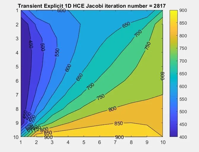
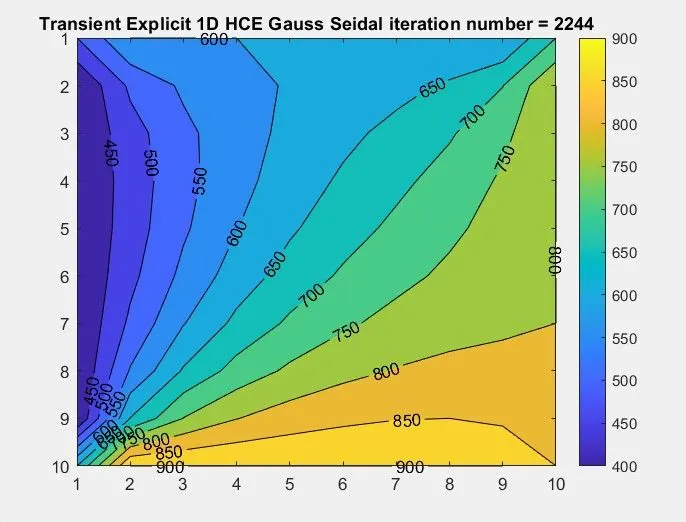
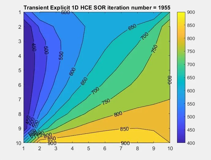
RESULTS:
OBSERVATION AND DISCUSSION FROM THE RESULT:
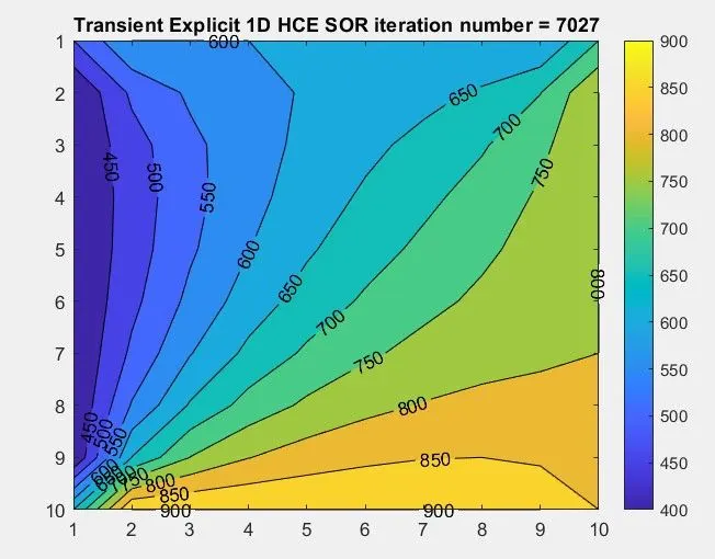
- It is observed from the result that SOR(Successive Over Relaxation) method takes least number of iterations and Gauss Jacobi method takes more number of iterations to converge to a final solution and Gauss Seidal method takes number of iterations inbetween 'Gauss Jacobi' and 'SOR'.
- From the iteration it has been concluded that in SOR method as the 'w' value(constant) decreases, the convergence rate is very low or it takes more number of iterations to get the optimal final solution compared to the Seidal and Jacobi also.
- For example, for w = 0.2 it took 7027 iterations to converge into final solution.
For w = 2.2, the obtained solution is unstable as shown below.
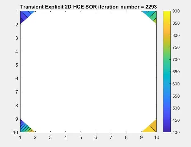
So it is necessary to give the 'w' value inbetween (1-1.5) to converge at faster rate.
CONCLUSION:
- It is concluded that for the faster convergence SOR with optimal 'w' (constant) value is chosen and converging rate is very slow for Jacobi method.
REFERENCES:
https://www.vedantu.com/maths/jacobian-method
https://mathworld.wolfram.com/SuccessiveOverrelaxationMethod.html