AIM:

To understand the concept of genetic algorithm and to write a code in MATLAB to optimise the stalagmite function and find the global maxima of the function.

GOVERNING EQUATION:

Equation for a stalagmite function,

f_x1 = (sin(5.1*pi*x+.5)).^6;

f_y1 = (sin(5.1*pi*y+.5)).^6;

f_x2 = exp((-4*log(2))*((x-.0667).^2)/(0.64));

f_y2 = exp((-4*log(2))*((y-.0667).^2)/(0.64));

f_xy = -f_x1.*f_x2.*f_y1.*f_y2;

where,

x = input_vector(1)=xx(i,j);

y = input_vector(2)=yy(i,j);

i,j = iteration values in the ‘for’ loop

OBJECTIVE OF THE PROJECT:

• To write a code in MATLAB to optimize the stalagmite function and find the global maxima of the function.
• To explain the concept of genetic algorithm and also explain the syntax for ‘ga’ in MATLAB in report.
• Plot graphs for all 3 studies and for F maximum vs no. of iterations.

BODY OF CONTENT:

Stalagmite:

A stalagmite is an upward-growing mound of mineral deposits that have precipitated from water dripping onto the floor of a cave. Most stalagmites have rounded or flattened tips. There are many other types of mineral formations found in caves.

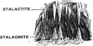
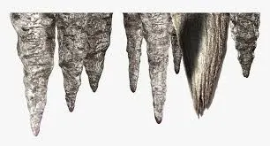
Here the optimum value for global maxima in stalagmite is determined using the concept of genetic algorithm discovered by Charles Darwin.

Optimization:

Optimization is the selection of a best element, with regard to some criterion, from some set of available alternatives. An optimization problem consists of maximizing or minimizing a real function by systematically choosing input values from within an allowed set and computing the value of the function. The generalization of optimization theory and techniques to other formulations constitutes a large area of applied mathematics.

Genetic Algorithm:

A genetic algorithm is a search heuristic that is inspired by Charles Darwin’s theory of natural evolution. This algorithm reflects the process of natural selection where the fittest individuals are selected for reproduction in order to produce offspring of the next generation.

Notion of Natural Selection

The process of natural selection starts with the selection of fittest individuals from a population. They produce offspring which inherit the characteristics of the parents and will be added to the next generation. If parents have better fitness, their offspring will be better than parents and have a better chance at surviving. This process keeps on iterating and at the end, a generation with the fittest individuals will be found.

This notion can be applied for a search problem. We consider a set of solutions for a problem and select the set of best ones out of them.

Five phases are considered in a genetic algorithm.

1. Initial population
2. Fitness function
3. Selection
4. Crossover
5. Mutation

Initial Population

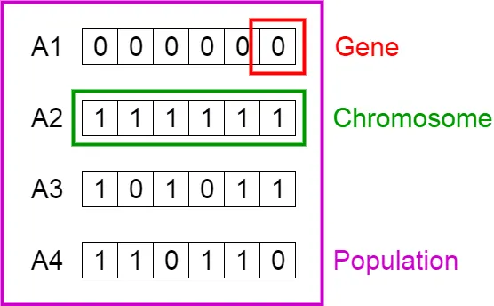
The process begins with a set of individuals which is called a Population. Each individual is a solution to the problem you want to solve.

An individual is characterized by a set of parameters (variables) known as Genes. Genes are joined into a string to form a Chromosome (solution).

In a genetic algorithm, the set of genes of an individual is represented using a string, in terms of an alphabet. Usually, binary values are used (string of 1s and 0s). We say that we encode the genes in a chromosome.

Fitness function:

The fitness function determines how fit an individual is (the ability of an individual to compete with other individuals). It gives a fitness score to each individual. The probability that an individual will be selected for reproduction is based on its fitness score.

Selection:

The idea of selection phase is to select the fittest individuals and let them pass their genes to the next generation.

Two pairs of individuals (parents) are selected based on their fitness scores. Individuals with high fitness have more chance to be selected for reproduction

Crossover:

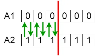
Crossover is the most significant phase in a genetic algorithm. For each pair of parents to be mated, a crossover point is chosen at random from within the genes.

For example, consider the crossover point to be 3 as shown below.

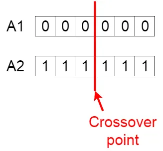
Offspring are created by exchanging the genes of parents among themselves until the crossover point is reached. The new offspring are added to the population.

Mutation

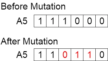
In certain new offspring formed, some of their genes can be subjected to a mutation with a low random probability. This implies that some of the bits in the bit string can be flipped.

Termination

The algorithm terminates if the population has converged (does not produce offspring which are significantly different from the previous generation). Then it is said that the genetic algorithm has provided a set of solutions to our problem.

Syntax for genetic algorithm:

x = ga(fun,nvars)

x = ga(fun,nvars,A,b)

x = ga(fun,nvars,A,b,Aeq,beq)

x = ga(fun,nvars,A,b,Aeq,beq,lb,ub)

x = ga(fun,nvars,A,b,Aeq,beq,lb,ub,nonlcon)

x = ga(fun,nvars,A,b,Aeq,beq,lb,ub,nonlcon,options)

x = ga(fun,nvars,A,b,[],[],lb,ub,nonlcon,IntCon)

x = ga(fun,nvars,A,b,[],[],lb,ub,nonlcon,IntCon,options)

x = ga(problem)

[x,fval] = ga(___)

[x,fval,exitflag,output] = ga(___)

[x,fval,exitflag,output,population,scores] = ga(___)

x = ga(fun,nvars,A,b) finds a local minimum x to fun, subject to the linear inequalities A*x ≤ b. ga evaluates the matrix product A*x as if x is transposed (A*x').

x = ga(fun,nvars,A,b,Aeq,beq) finds a local minimum x to fun, subject to the linear equalities Aeq*x = beq and A*x ≤ b. (Set A=[] and b=[] if no linear inequalities exist.) ga evaluates the matrix product Aeq*x as if x is transposed (Aeq*x').

x = ga(fun,nvars,A,b,Aeq,beq,lb,ub) defines a set of lower and upper bounds on the design variables, x, so that a solution is found in the range lb ≤ x ≤ ub. (Set Aeq=[] and beq=[] if no linear equalities exist.)

x = ga(fun,nvars,A,b,Aeq,beq,lb,ub,nonlcon) subjects the minimization to the constraints defined in nonlcon. The function nonlcon accepts x and returns vectors C and Ceq, representing the nonlinear inequalities and equalities respectively. ga minimizes the fun such that C(x) ≤ 0 and Ceq(x) = 0. (Set lb=[] and ub=[] if no bounds exist.)

x = ga(fun,nvars,A,b,Aeq,beq,lb,ub,nonlcon,options) minimizes with the default optimization parameters replaced by values in options. (Set nonlcon=[] if no nonlinear constraints exist.) Create options using optimoptions.

x = ga(fun,nvars,A,b,[],[],lb,ub,nonlcon,IntCon) or x = ga(fun,nvars,A,b,[],[],lb,ub,nonlcon,IntCon,options) requires that the variables listed in IntCon take integer values.

Code:

close all
clear all
clc

x = linspace(0,0.6,150);
y = linspace(0,0.6,150);
num_cases = 50
[xx yy] = meshgrid(x,y);

% Evaluating the stalagmite function
for i = 1:length(xx);
    for j = 1:length(yy);
        input_vector(1)=xx(i,j);
        input_vector(2)=yy(i,j);
        f(i,j) = stalagmite(input_vector);
    end
end
 tic
%study 1 - statistical behaviour
for i = 1:num_cases
    [inputs, fopt(i)] = ga(@stalagmite, 2);
    xopt(i) = inputs(1);
    yopt(i) = inputs(2);
end

study1_time = toc

figure(1)
subplot(2,1,1)
hold on
surfc(x, y, -f)
shading interp
plot3(xopt,yopt,-fopt,'marker','o','markersize',5,'markerfacecolor','r')
title('unbounded inputs')
subplot(2,1,2)
plot(-fopt)
xlabel('iterations')
ylabel('function maximun')

tic
%study 2 - Statistical behaviour - with upper and lower bounds
for i = 1:num_cases
    [inputs, fopt(i)] = ga(@stalagmite,2,[],[],[],[],[0;0],[.6;.6]);
    xopt(i) = inputs(1);
    yopt(i) = inputs(2);
end
study2_time = toc

figure(2)
subplot(2,1,1)
hold on
surfc(x, y, -f)
shading interp
plot3(xopt,yopt,-fopt,'marker','o','markersize',5,'markerfacecolor','r')
title('bounded inputs 2')
subplot(2,1,2)
plot(-fopt)
xlabel('iterations')
ylabel('Function maximum')

% Study 3 increasing GA iterations
options = optimoptions('ga');
options = optimoptions(options, 'populationsize', 170);

tic
for i = 1:num_cases
    [inputs, fopt(i)] = ga(@stalagmite,2,[],[],[],[],[0;0],[0.1;0.1],[],[],options);
    xopt(i) = inputs(1);
    yopt(i) = inputs(2);
end
study3_time = toc
figure(3)
subplot(2,1,1)
hold on
surfc(x, y, -f)
shading interp
plot3(xopt,yopt,-fopt,'marker','o','markersize',5,'markerfacecolor','r')
title('bounded inputs')
subplot(2,1,2)
plot(-fopt)
xlabel('iterations')
ylabel('Function maximum')

Supplymentary code:

Code for Stalagmite function:

function [f_xy] = stalagmite(input_vector);

x = input_vector(1);
y = input_vector(2);

f_x1 = (sin(5.1*pi*x+.5)).^6;
f_y1 = (sin(5.1*pi*y+.5)).^6;
f_x2 = exp((-4*log(2))*((x-.0667).^2)/(0.64));
f_y2 = exp((-4*log(2))*((y-.0667).^2)/(0.64));
f_xy = -f_x1.*f_x2.*f_y1.*f_y2;
end

Explanation:

Initially the ‘x’ and ‘y’ values are assigned using the ‘linspace’ command where the values start from 0 to 0.6 with 150 intervals.

To proceed this program the 3D plot is required, so the ‘meshgrid’ command is used to get 2D plot of ‘X’ and ‘Y’ axis. Initially the number of case studies is assigned as 50 which is assigned as ‘num_cases’ = 50.

Evaluating the stalagmite function:

Then, the stalagmite function is obtained by the following governed equation as shown above. This is created in the separate stalagmite file name and we take the data from the above. Here the nested ‘for’ loop is created and for each ‘x’ and ‘y’ value, using stalagmite function the stalagmite is created. ‘ga’ finds a local unconstrained minimum, x, to the objective function, fun.

x = ga(fun,nvars)

where, ‘nvars’ represents the number of degign variables of the function.

Case study 1- Statistical behavior for unbounded values:

Here initially the iteration value is assigned as 50.(which is num_cases=50 here). For 50 iterations the optimum maximum value for the stalagmite function is predicted without any boundary conditions. The time is recorded for the program to execute using ‘tic’ and ‘toc’ command.

Then 3D plotting is done using ‘plot3’ command in the subplot of 1^st row.

Syntax:plot3(X,Y,Z)

Subplot:

'subplot(m,n,p)' divides the current figure into an m-by-n grid and creates axes in the position specified by p. MATLAB® numbers subplot positions by row. The first subplot is the first column of the first row, the second subplot is the second column of the first row, and so on. If axes exist in the specified position, then this command makes the axes the current axes.

Syntax:subplot(m,n,p)

Surfc:

surfc(X,Y,Z) creates a three-dimensional surface plot with a contour plot underneath. A surface plot is a three-dimensional surface that has solid edge colors and solid face colors. The function plots the values in matrix Z as heights above a grid in the x-y plane defined by X and Y. The color of the surface varies according to the heights specified by Z. Here the ‘z’ value represents the peak of the stalagmite. The negative sign of the function represents the maximum value of the stalagmite since the ‘ga’ command represents the minima of the function. So negative value is given.

Syntax: surfc(X,Y,Z)

shading interp:

'shading interp' varies the color in each line segment and face by interpolating the color map index or true color value across the line or face.

Then the title for the figure is given using title command.

The subplot1 specifies the 3D figure of the stalagmite function whereas the subplot2 specifies the optimum global maximum value for the given iterations.

The ‘xlabel’ and ‘ylabel’ command is used to give the title for the ‘x’ and ‘y’ axis in the subplot2.

Then, the results are as shown below and it took 11.554 seconds to execute the results.

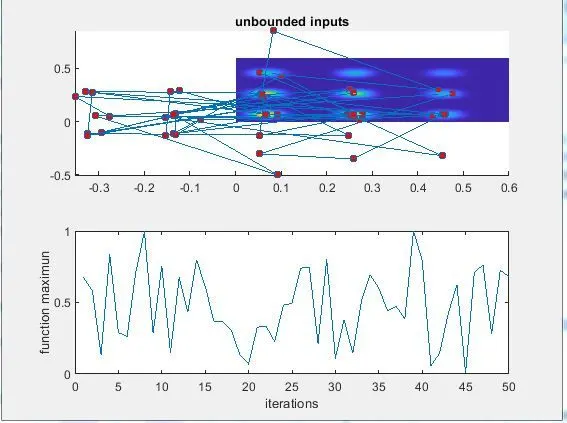
Here, the plot is obtained as random sampling with multiple points as maxima for each iterations. So this can’t be the optimum value for the given input. Thus it has to be corrected by giving boundary conditions in ‘ga’ command. The boundary conditions are given as [0,0] to [0.6,0.6] and this is proceeded in case 2 study.

The result obtained in case 2 study [Statistical behaviour - with upper and lower bounds] is as shown below and it took 11.3232 seconds to execute the result.

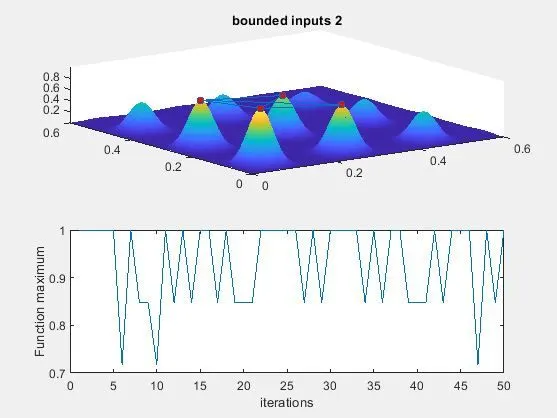
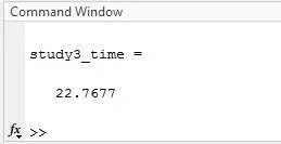
Even in case study 2, the there are 4 optimal function points of maxima in stalagmite which is constrained from multiple points to 4 points. So in order to constrain to a single point of optimal maxima, the population size is increased to 170 and the boundary condition are further reduced to [0,0] to [0.1,0.1] and program is executed in case study 3. The results are as shown below and it took 22.7677 seconds to execute the program.

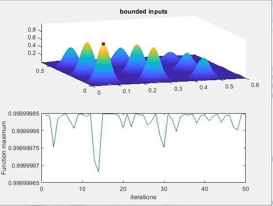
Finally in case study 3, the single point for optimal global maxima for a stalagmite function is obtained by increasing the iteration and population size.

Errors faced:

• In the supplementary program, the function name is assigned as ‘inputs’ instead of ‘f_xy’. So while calling the function, the error shows as ’The output argument “inputs” is not assigned during the call to “stalagmite”.

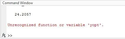
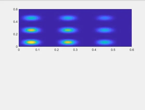
• In the case study 3, the initiation of ‘yopt’ is not assigned which was mistakenly assigned as ‘xopt’ and during calling in the ‘plot3’ command, the program couldn’t recognize the function ‘yopt’ and it displayed in the command window as “unrecognized function or variable ‘yopt’”. So the subplot is not displayed in the figure 3 since the ‘yopt’ command is unrecognized. Then the mistake was found and corrected.

Conclusion:

Thus the code to optimize the stalagmite function and find the global maxima of the function in MATLAB is done and the final optimized result for global maxima is found to be 0.999999. From the above coding, it has been concluded that the optimal value for stalagmite function maxima can be determined by increasing the population size and number of iterations with constrained boundary inputs.