Week 7 - Simulation of a 1D Super-sonic nozzle flow simulation using Macormack Method

AIM:

simulation of a 1D supersonic Nozzle flow simulation useing Macormack method.

THEORY:

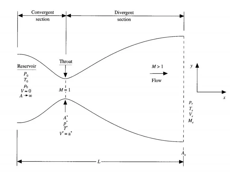
the flow in the convergent divergent nozzle is isentropic flow. the inlet of convergent nozzle is connected to reserovoir. the flow in the convergent portion is subsonic flow. the flow in the throat portion is sonic flow and the flow in the divergent portion is supersonic flow. we will study how the primitive variables (density,velocity,temperature,pressure,mass flow rate) are vary along the length of the nozzzle by using governing equations.

Governing equations:

the governing equations used to solve the above problem are

• continuity equation
• momentum equation
• energy equation

To derive the equations we use two methods

1.conserrvative method

2.non conservative method

1.conservative method:

let us take a closed volume drawn within a finite region of flow. This volume defines a 'control volume'. this control volume is fixed in space with in the fluid moving through out.from this closed volume we are going to obtain the governing equations.

the govering equations obtained from this method are

continuity equation :

`(∂(ρ'A'))/(∂t ') + (∂(ρ'A'V'))/(∂x ') = 0`

momentum equation :

`(∂(ρ'A'V'))/(∂t ') + (∂[ρ^' A^' V'^2+(1/γ)P'A'])/(∂x ') = 1/γ P'(∂A ')/(∂x ')`

energy equation :

`(∂[ρ'(e^'/(γ-1)+(γ )/2 〖V^̍〗^2 )A'])/(∂t ') + (∂[ρ'(e^'/(γ-1)+(γ )/2 〖V^̍〗^2 )A'V'+P'A'V'])/(∂x ') = 0`

as we know that the above primitive variables are non dimensional numbers. also we know that e = cv.t, where as cv is constant as energy(e) so we can write e ' as t '

`(∂[ρ'(t^'/(γ-1)+(γ )/2 〖V^̍〗^2 )A'])/(∂t ') + (∂[ρ'(t^'/(γ-1)+(γ )/2 〖V^̍〗^2 )A'V'+P'A'V'])/(∂x ') = 0`

2.Non Conservative method :

let us image the closed volume in the finite region of fluid flow.This closed volume definrs 'control volume'. This control volume is moving with the fluid, such that same fluid particles are always inside the control volume. From this moving control volume we are going to obtain th governing equations.

Continuity equation :

`(∂ρ ')/(∂t ') = -ρ' (∂V ')/(∂x ') - ρ'V'(∂(〖ln A '〗⁡))/(∂x ') - V'(∂ρ ')/(∂x ')`

Momentum equation:

`(∂V ')/(∂t ') = -V' (∂V ')/(∂x ') - 1/γ((∂t ')/(∂x ') + (t ')/(ρ ') (∂ρ ')/(∂x '))`

Energy equation :

`(∂t ')/(∂x ') = -V' (∂t ')/(∂x ') - (γ-1) t^' [(∂V ')/(∂x ') + V'(∂(〖ln A '〗⁡))/(∂x ')]`

objectives :

we need to show the following plots

a. Steady-state distribution of primitive variables inside the nozzle

b. Time-wise variation of the primitive variables

c. Variation of Mass flow rate distribution inside the nozzle at different time steps during the time-marching process

d. Comparison of Normalized mass flow rate distributions of both forms

Main code:

clear all
close all
clc

%inputs
n = 31;
x = linspace(0,3,n);
dx = x(2)-x(1);
gama = 1.4;
throat = (n-1)/2;
%courant number
c = 0.5;
%mass flow rate
Q_analytical = 0.579.*ones(1,n);

%non conservative form
 [Q_nc,rho_nc,v_nc,t_nc,P_nc,M_nc,rho_throat_nc,v_throat_nc,t_throat_nc,P_throat_nc,M_throat_nc] = non_conservative(n,x,dx,gama,throat,Q_analytical);

%conservative form
 [Q_c,rho_c,v_c,t_c,P_c,M_c,rho_throat_c,v_throat_c,t_throat_c,P_throat_c,M_throat_c] = conservative(n,x,dx,gama,throat,c,Q_analytical);
 figure(7)
 plot(x,Q_nc(1400,:),'r')
 hold on
 plot(x,Q_c(1400,:),'b')
 hold on
 plot(x,Q_analytical,'g')
 xlabel('length of nozzle')
 ylabel('mass flow rate')
 legend('non conservative form','conservative form','exact mass flow rate')
 title_text = sprintf('normalized mass flow distribution of both conservative and non conservative form for 31 nodes');
 title(title_text)

non conservative form function code :

function [Q_nc,rho_nc,v_nc,t_nc,P_nc,M_nc,rho_throat_nc,v_throat_nc,t_throat_nc,P_throat_nc,M_throat_nc] = non_conservative(n,x,dx,gama,throat,c,Q_analytical) 
%initial profiles
%density
rho_nc = 1-0.3146*x;
%temperature
t_nc = 1-0.2314*x;
%velocity
v_nc = (0.1+1.09*x).*t_nc.^(1/2);
%area
a = 1+2.2*(x-1.5).^2;

rho_old_nc = rho_nc;
v_old_nc = v_nc;
t_old_nc = t_nc;
%time steps
nt = linspace(1,1400,1400);
%time loop
for i = 1:length(nt)
    dt=min(c*dx./(sqrt(t_nc)+v_nc));
    %predictor method
    for j = 2:n-1
        %drho/dt_p =-rho*(dv/dx)-rho*v*(loga/dx)-v*drho/dx
        dvdx = (v_old_nc(j+1)-v_old_nc(j))/dx;
        drhodx = (rho_old_nc(j+1)-rho_old_nc(j))/dx;
        dtdx = (t_old_nc(j+1)-t_old_nc(j))/dx;
        dlogadx = (log(a(j+1))-log(a(j)))/dx;
        
        %continuity equation
        drhodt_p(j) = (-rho_old_nc(j)*dvdx)-(rho_old_nc(j)*v_old_nc(j)*dlogadx)-(v_old_nc(j)*drhodx);
        %momentum equation
        dvdt_p(j) = (-v_old_nc(j)*dvdx)-(1/gama)*(dtdx+(t_old_nc(j)/rho_old_nc(j)*drhodx));
        %energy equation
        dtdt_p(j) = (-v_old_nc(j)*dtdx)-(gama-1)*t_old_nc(j)*(dvdx+(v_old_nc(j)*dlogadx));
    
        %solution updates
        v_nc(j) = v_old_nc(j)+dvdt_p(j)*dt;
        rho_nc(j) = rho_old_nc(j)+drhodt_p(j)*dt;
        t_nc(j) = t_old_nc(j)+dtdt_p(j)*dt;
        %pressure(j) = rho_old(j)*t_old(j);
    end
    
    %corrector method
      for j = 2:n-1
        %drho/dt_p =-rho*(dv/dx)-rho*v*(loga/dx)-v*drho/dx
        dvdx = (v_nc(j)-v_nc(j-1))/dx;
        drhodx = (rho_nc(j)-rho_nc(j-1))/dx;
        dtdx = (t_nc(j)-t_nc(j-1))/dx;
        dlogadx = (log(a(j))-log(a(j-1)))/dx;
        
        %continuity equation
        drhodt_c(j) = (-rho_nc(j)*dvdx)-(rho_nc(j)*v_nc(j)*dlogadx)-(v_nc(j)*drhodx);
        %momentum equation
        dvdt_c(j) = (-v_nc(j)*dvdx)-(1/gama)*(dtdx+(t_nc(j)/rho_nc(j)*drhodx));
        %energy equation
        dtdt_c(j) = (-v_nc(j)*dtdx)-(gama-1)*t_nc(j)*(dvdx+(v_nc(j)*dlogadx));
      end
      
      %compute average time derivative
      drhodt = 0.5*(drhodt_p+drhodt_c);
      dvdt = 0.5*(dvdt_p+dvdt_c);
      dtdt = 0.5*(dtdt_p+dtdt_c);
      
      %final solution
      for k = 2:n-1
          rho_nc(k) = rho_old_nc(k)+drhodt(k)*dt;
          v_nc(k)= v_old_nc(k)+dvdt(k)*dt;
          t_nc(k) = t_old_nc(k)+dtdt(k)*dt;
      end

      %apply boundary conditions
      %inlet
      v_nc(1) = 2*v_nc(2)-v_nc(3);
      
      %outlet
      v_nc(n) = 2*v_nc(n-1)-v_nc(n-2);
      rho_nc(n) = 2*rho_nc(n-1)-rho_nc(n-2);
      t_nc(n) = 2*t_nc(n-1)-t_nc(n-2);
      for l = 1:n
          %pressure = P
          P_nc(l) = rho_nc(l)*t_nc(l);
          %Mach number = M
          M_nc(l) = v_nc(l)./(t_nc(l))^0.5;
          
      end
      %mass flow rate at different steps
      Q_nc(i,:) = rho_nc.*a.*v_nc; 
      
      %the primitive values at throat
      t_throat_nc(i)=t_nc(throat);
      rho_throat_nc(i) = rho_nc(throat);
      v_throat_nc(i) =v_nc(throat);
      P_throat_nc(i) = P_nc(throat);
      M_throat_nc(i) = M_nc(throat);
         
       %updating old values
        rho_old_nc = rho_nc;
        v_old_nc = v_nc; 
        t_old_nc = t_nc;

end
%plotting
%plot on non conservative form-mass flow rate after different time steps
figure(1)
plot(x,Q_analytical,'m')
hold on
plot(x,Q_nc(1,:),'r')
hold on
plot(x,Q_nc(100,:),'y')
hold on
plot(x,Q_nc(300,:),'g')
hold on
plot(x,Q_nc(700,:),'c')
hold on
plot(x,Q_nc(1000,:),'k')
hold on
plot(x,Q_nc(1400,:),'b')
xlabel('length of nozzle')
ylabel('mass flow rate at different time steps')
legend('anaytical value','after 1 time step','after 100 time steps','after 300 time steps','after 700 time steps','after 1000 time steps','after 1400 time steps')
title_text = sprintf('non conservative form-mass flow rate after different time steps');
title(title_text)

%plot on non conservative form-steady state position of primitive variables
figure(2)
subplot(6,1,1)
plot(x,rho_nc,'r')
xlabel('length of nozzle')
ylabel('density')
legend('density')
title_text = sprintf('non conservative form-steady state position of primitive variables');
title(title_text)
subplot(6,1,2)
plot(x,v_nc,'b')
xlabel('length of nozzle')
ylabel('velocity')
legend('velocity')
subplot(6,1,3)
plot(x,t_nc,'g')
xlabel('length of nozzle')
ylabel('temperature')
legend('temperature')
subplot(6,1,4)
plot(x,P_nc,'c')
xlabel('length of nozzle')
ylabel('pressure')
legend('pressure')
subplot(6,1,5)
plot(x,M_nc,'k')
xlabel('length of nozzle')
ylabel('mach number')
legend('mach number')
subplot(6,1,6)
plot(x,Q_nc(1400,:),'y')
xlabel('length of nozzle')
ylabel('mass flow rate')
legend('mass flow rate') 

%plot on conservative form-time wise variation at node 15
figure(3)
plot(nt,rho_throat_nc,'r')
hold on
plot(nt,v_throat_nc,'b')
hold on
plot(nt,t_throat_nc,'g')
hold on
plot(nt,P_throat_nc,'c')
hold on
plot(nt,M_throat_nc,'k')
hold on
plot(nt,Q_nc(:,15),'y')
legend('density','velocity','temperature','pressure','mach number','mass flow rate')
xlabel('number of iterations')
ylabel('non dimension values')
title_text = sprintf('non conservative form-time wise variation at node 15');
title(title_text)
end

conservative form function code:

function [Q_c,rho_c,v_c,t_c,P_c,M_c,rho_throat_c,v_throat_c,t_throat_c,P_throat_c,M_throat_c] = conservative( n,x,dx,gama,throat,c,Q_analytical)
%initial profiles

%density
%temperatue
for i= 1:length(x)
    if x(i)<=0.5
        rho_c(i) = 1;
        t_c(i) = 1;
    elseif x(i)> 0.5 && x(i) < 1.5
         rho_c(i) = 1- 0.366*(x(i) - 0.5); 
         t_c(i) = 1-0.167*(x(i) - 0.5);
    else
        rho_c(i) = 0.634 - 0.3879*(x(i) - 1.5);
        t_c(i) = 0.833 - 0.3507*(x(i) - 1.5);
    end
end
%area
a = 1+2.2*(x-1.5).^2;
%velocity
v_c = 0.59./(rho_c.*a);
%define of elements
U1 = rho_c.*a;
U2 = rho_c.*a.*v_c;
U3 = rho_c.*((t_c./(gama-1))+gama/2*v_c.^2).*a;
U1_old = U1;
U2_old = U2;
U3_old = U3;
%time steps
nt = linspace(1,1400,1400);

%time loop
for h = 1:length(nt)
    dt=min(c*dx./(sqrt(t_c)+v_c));
%prediction method
 for j = 1:n
     F1(j) = U2_old(j);
     F2(j) = U2_old(j)^2/U1_old(j) + ((gama-1)/gama)*(U3_old(j)-(gama/2)*U2_old(j)^2/U1_old(j));
     F3(j) = (((gama*U2_old(j)*U3_old(j))/U1_old(j))-gama*(gama-1)*0.5*U2_old(j)^3/U1_old(j)^2);
 end
 for i = 2:n-1
    dadx(i) = (a(i+1)-a(i))/dx;
    j2(i) = (1/gama)*rho_c(i)*t_c(i)*dadx(i);
end
 for k = 2:n-1
     dU1dt_p(k) = -(F1(k+1)-F1(k))/dx;
     dU2dt_p(k) = -(F2(k+1)-F2(k))/dx + j2(k);
     dU3dt_p(k) = -(F3(k+1)-F3(k))/dx;
     
     %solution update
     U1(k) = U1_old(k)+ dU1dt_p(k)*dt;
     U2(k) = U2_old(k)+ dU2dt_p(k)*dt;
     U3(k) = U3_old(k)+ dU3dt_p(k)*dt;
     %prediction density
     rho_c(k) = U1(k)/a(k);
     %predition velocity
     v_c(k) = U2(k)/U1(k);
     %prediction temperature
     t_c(k) = (gama-1)*((U3(k)/U1(k)-gama/2*(U2(k)/U1(k))^2));
 end
 
 %correction method
  for j = 1:n
     F1(j) = U2(j);
     F2(j) = U2(j)^2/U1(j) + ((gama-1)/gama)*(U3(j)-(gama/2)*U2(j)^2/U1(j));
     F3(j) = (((gama*U2(j)*U3(j))/U1(j))-gama*(gama-1)*0.5*U2(j)^3/U1(j)^2);
  end
 for i = 2:n-1
    dadx(i) = (a(i)-a(i-1))/dx;
    j2(i) = (1/gama)*rho_c(i)*t_c(i)*dadx(i);
end
 for l = 2:n-1
      dU1dt_c(l) = -(F1(l)-F1(l-1))/dx;
      dU2dt_c(l) = -(F2(l)-F2(l-1))/dx + j2(l);
      dU3dt_c(l) = -(F3(l)-F3(l-1))/dx;
 end
       %compute average time derivative
      dU1dt = 0.5*(dU1dt_p + dU1dt_c);
      dU2dt = 0.5*(dU2dt_p + dU2dt_c);
      dU3dt = 0.5*(dU3dt_p + dU3dt_c);
  for m = 2:n-1     
       U1(m) = U1_old(m) + dU1dt(m)*dt;
       U2(m) = U2_old(m) + dU2dt(m)*dt;
       U3(m) = U3_old(m) + dU3dt(m)*dt;
       %final density
       rho_c(m) = U1(m)/a(m);
       %final velocity
       v_c(m) = U2(m)/U1(m);
       %final temperature
       t_c(m) = (gama-1)*((U3(m)/U1(m)-gama/2*(U2(m)/U1(m))^2));
       %final pressure
  end
       %apply boundary conditions
       %inlet
       U1(1) = rho_c(1)*a(1);
       U2(1) = 2*U2(2)-U2(3);
       U3(1) = U1(1)*((t_c(1)/(gama-1))+(gama/2)*v_c(1)^2);
       rho_c(1) = U1(1)/a(1);
       v_c(1) = U2(1)/U1(1);
       t_c(1) = (gama-1)*((U3(1)/U1(1)-gama/2*(U2(1)/U1(1))^2));
       
       %outlet
       U1(n) = 2*U1(n-1)-U1(n-2);
       U2(n) = 2*U2(n-1)-U2(n-2);
       U3(n) = 2*U3(n-1)-U3(n-2);
       t_c(n) = (gama-1)*((U3(n)/U1(n)-gama/2*(U2(n)/U1(n))^2));
       rho_c(n) = U1(n)/a(n);
       v_c(n) = U2(n)/U1(n);
   
        %pressure = P
        P_c = rho_c.*t_c(l);
        %Mach number = M
        M_c = v_c./(t_c).^0.5;
   
        %mass flow rate at different steps
        Q_c(h,:) = rho_c.*a.*v_c;
       
        %primitive variables at throat
        t_throat_c(h) = t_c(throat);
        rho_throat_c(h) = rho_c(throat);
        v_throat_c(h) = v_c(throat);
        P_throat_c(h) = P_c(throat);
        M_throat_c(h) = M_c(throat);
       
        %update old values
        U1_old = U1;
        U2_old = U2;
        U3_old = U3;
end    
       
%plotting
%plot on conservative form-mass flow rate after different time steps
figure(4)
plot(x,Q_analytical,'m')
hold on
plot(x,Q_c(1,:),'r')
hold on
plot(x,Q_c(100,:),'y')
hold on
plot(x,Q_c(300,:),'g')
hold on
plot(x,Q_c(700,:),'c')
hold on
plot(x,Q_c(1000,:),'k')
hold on
plot(x,Q_c(1400,:),'b')
xlabel('length of nozzle')
ylabel('mass flow rate at different time steps')
legend('anaytical value','after 1 time step','after 100 time steps','after 300 time steps','after 700 time steps','after 1000 time steps','after 1400 time steps')
title_text = sprintf('conservative form-mass flow rate after different time steps');
title(title_text)

%plot on non conservative form-steady state position of primitive variables
figure(5)
subplot(6,1,1)
plot(x,rho_c,'r')
xlabel('length of nozzle')
ylabel('density')
legend('density')
title_text = sprintf('conservative form-steady state position of primitive variables');
title(title_text)
subplot(6,1,2)
plot(x,v_c,'b')
xlabel('length of nozzle')
ylabel('velocity')
legend('velocity')
subplot(6,1,3)
plot(x,t_c,'g')
xlabel('length of nozzle')
ylabel('temperature')
legend('temperature')
subplot(6,1,4)
plot(x,P_c,'c')
xlabel('length of nozzle')
ylabel('pressure')
legend('pressure')
subplot(6,1,5)
plot(x,M_c,'k')
xlabel('length of nozzle')
ylabel('mach number')
legend('mach number')
subplot(6,1,6)
plot(x,Q_c(1400,:),'y')
xlabel('length of nozzle')
ylabel('mass flow rate')
legend('mass flow rate')

%plot on conservative form-time wise variation at node 15
figure(6)
plot(nt,rho_throat_c,'r')
hold on
plot(nt,v_throat_c,'b')
hold on
plot(nt,t_throat_c,'g')
hold on
plot(nt,P_throat_c,'c')
hold on
plot(nt,M_throat_c,'k')
hold on
plot(nt,Q_c(:,15),'y')
legend('density','velocity','temperature','pressure','mach number','mass flow rate')
xlabel('number of iterations')
ylabel('non dimension values')
title_text = sprintf('conservative form-time wise variation at node 15');
title(title_text)
end

after running the above code, we are going get the below plots:

figures 1,2,3 are obtained from non conservative form

figure(1)-

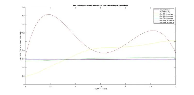
this figure represents how the mass flow rate flows along the length of the nozzle at different time steps. also we can see that the analytical value of mass flow rate line almost closed with with the mass flow rate lines after 700 time steps.

figure(2)-

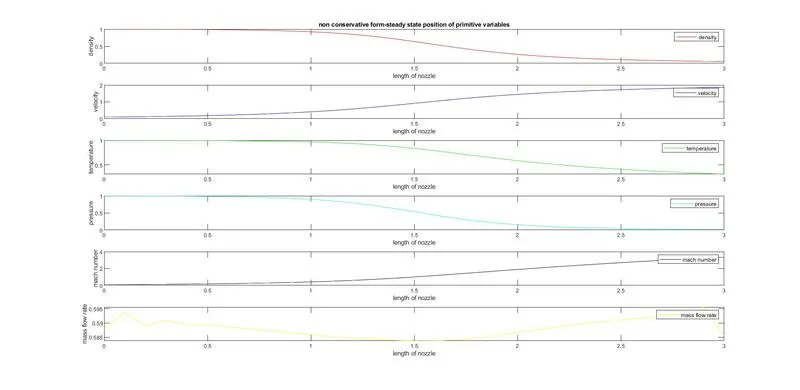
this figure represents how the primative variables reached to steady state after 1400 time steps along the length of the nozzle.

figure(3)-

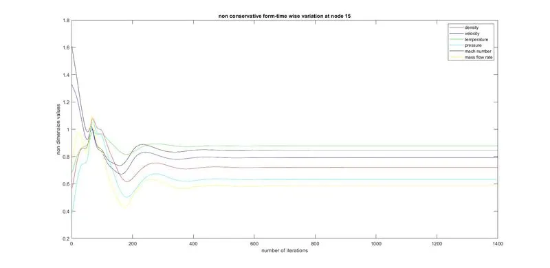
this figure represents how the primitive variables varies at node 15,that is at throat at each time step. from the figure we can see that all the primitive variables reached to steady state after around 500 time steps.

figures 4,5,6 are obtained from the conservative form

figure(4)-

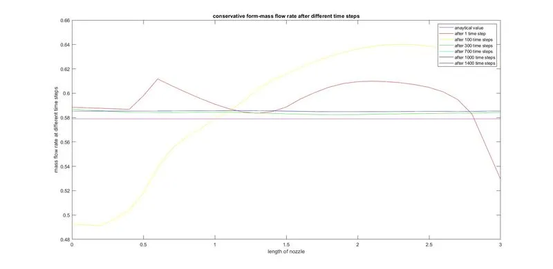
this figure represents how the mass flow rate flows along the length of the nozzle at different time steps. also we can see that the analytical value of mass flow rate line almost closed with with the mass flow rate lines after 700 time steps. but compared to non conservative form , from the conservative form the analytical value of mass flow rate line is much more closed to the mass flow rate lines after 700 time steps.

figure(5)-

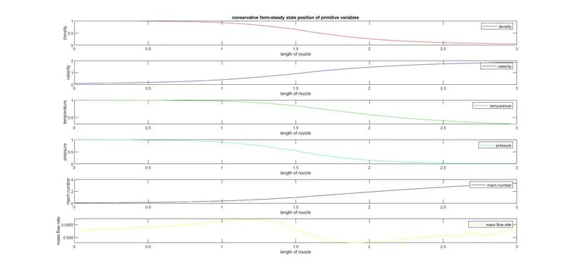
this figure represents how the primative variables reached to steady state after 1400 time steps along the length of the nozzle.

figure(6)-

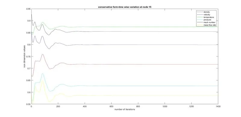
this figure represents how the primitive variables varies at node 15,that is at throat at each time step. from the figure we can see that all the primitive variables reached to steady state after around 400 time steps. from this we can say that by using conservative method the primitive variables reached to steady state faster compared to non conservative method.

Grid independency test:

grid independency test means that if we change the number of grid points, how the primitive variable values from both conservative form and non conservative form gets closed to analytical values at node 15 that is at throat of the nozzle.

figure(7)-

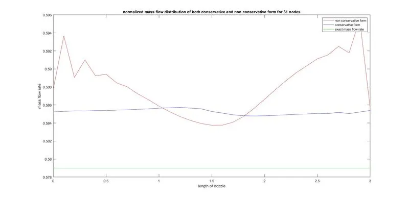
the above figure represents how the mass flow rate varies along the length of the nozzle by using both conservative and non conservative forms with 31 nodes. and also we can see that mass flow rate line of conservative form is reached to most efficient steady state position and this line is so closed with the analytical mass flow rate line.

figure(8)-

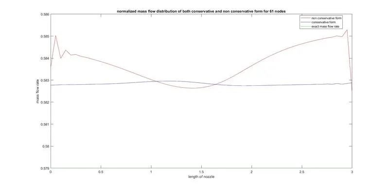
the above figure represents how the mass flow rate varies along the length of the nozzle by using both conservative and non conservative forms with 61 nodes. but compared with31 nodes, with 61 nodes the mass flow rate values using both conservative and non conservative formreached so much close to analytical mass flow rate value.

below i am going to show the mass flow rate values

mass flow rate

analytical value - 0.579

conservative form(with 31 nodes) - 0.5854

non conservative form(with 31 nodes) - 0.584

conservative form(with 61 nodes) - 0.5829

non conservative form(with 61 nodes) - 0.5825

from this we can conclude with with the increase in number of grid points, the primitive variables are almost so close to analytical value.