Week 7: Shock tube simulation project

AIM:

Shock tube simulation project

objectives:

• Setup a transient shock tube simulation
• Plot the pressure and temperature history in the entire domain - Explain the result
• Plot the cell count as a function of time - Explain the result

theory:

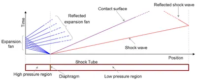
In a shock tube, the sudden expansion of a gas at high pressure into a gas at low pressure produces a plane shock wave that then propagates through a long closed tube. The shock wave is used to produce a rapid increase in the pressure and the temperature of a reactive mixture. In most shock tubes, the shock wave is reflected at the end of the tube and produces during its way back a second rise in temperature. This technique is mainly used to study elementary steps, as well as pyrolysis and high-temperature autoignition in very dilute mixtures.

the shock tube is a long tube of uniform cross section and with uniform interna dimensions. the diaphragm separates the high pressure driver section from low pressure driven section. the material of the diaphragm and its thicjness are dictated by the pressure ratio between the sections. on abrupt rupturing of diaphragm, pressure waves spread out diaphragm section comes together to form shock front which propagates into the low pressure region. the wave diagram of the shock tube after diaphragm rupture is given in below figure

geometry:

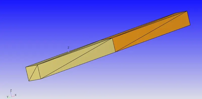
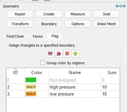
now i have named the above geometry using boundary flagging tool. the left box is named as high pressure and the right box is named as low pressure. in between there is diamphragm was created. instead of diaphragm we use events tool in the converge.

case setup:

application type: time beased

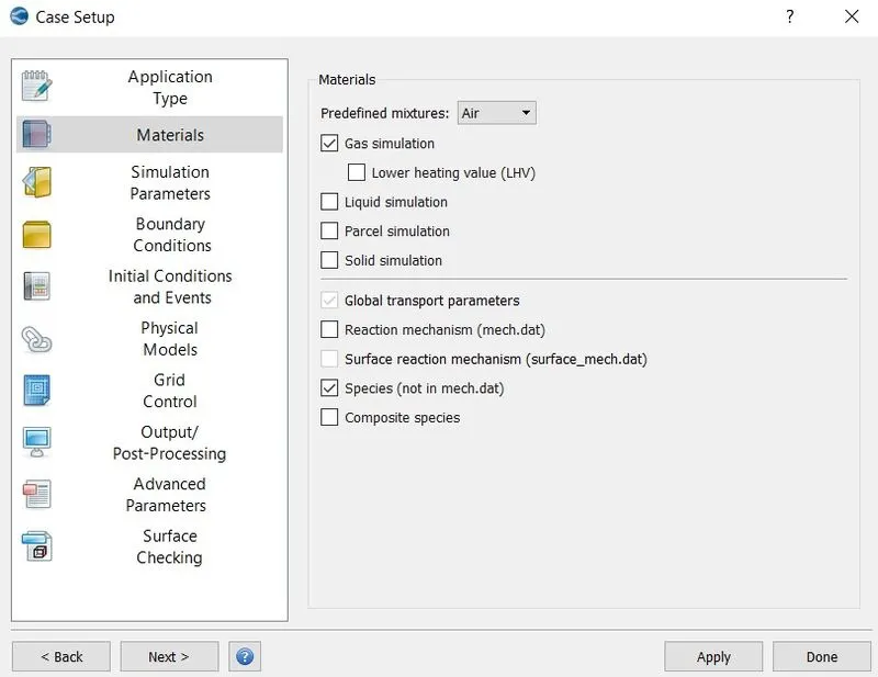
materials: air

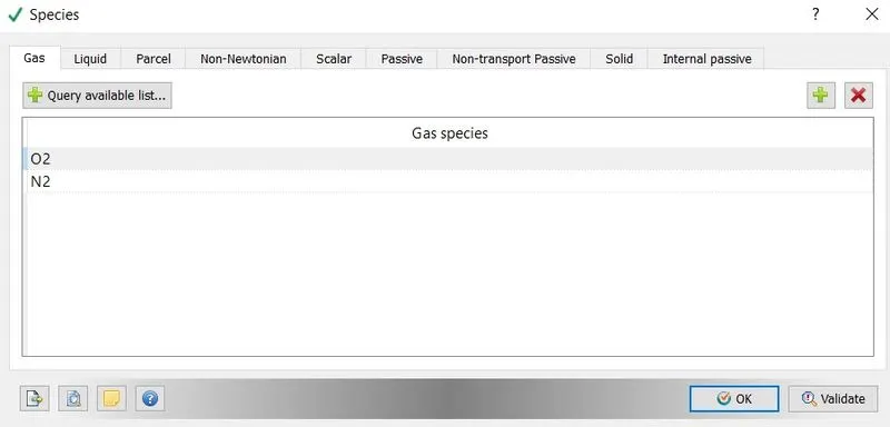
click on gas simulation as the air is gaseous state and click on species to calcuate how the mass fraction of N2 and O2 are changing along the flow.

species-

simulation parameters:

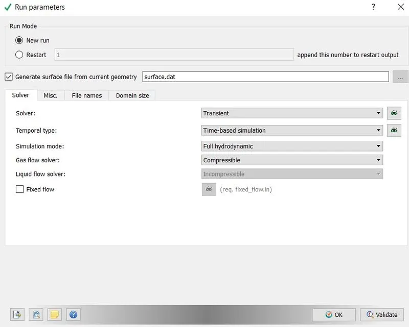
run parameters-

i am running the somulation using transient state solver because here the throttle has to rotate with time. the primitive variables gets changes with time. so to capture them i have used transient state solver. full hydrodynamic simulation mode is used for simple geometries.

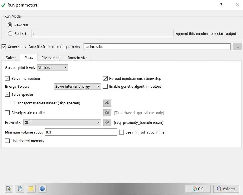
we have click on steady state monitor only for the steady state problems only.

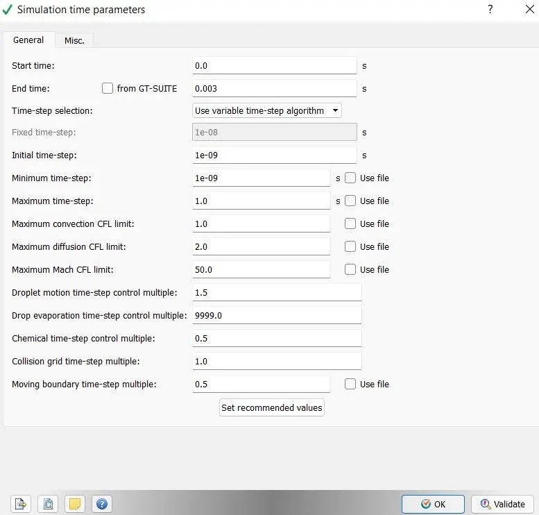
simulation time parameters-

the maximum convection cfl number should always be less than or equal to 1. so that solution would converge otherwise solution gets blown up.to calculate the end time, i have used the following procedure.

solver parameters-

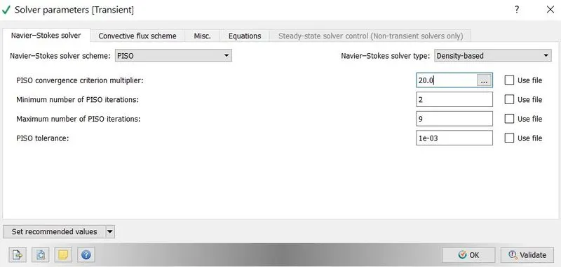
density based solver is used here

initial conditions and events:

regions and initialization-

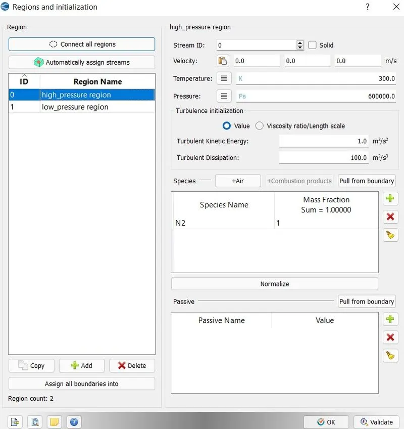
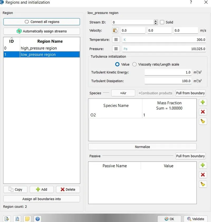
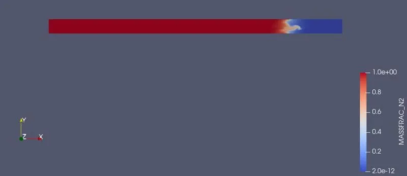
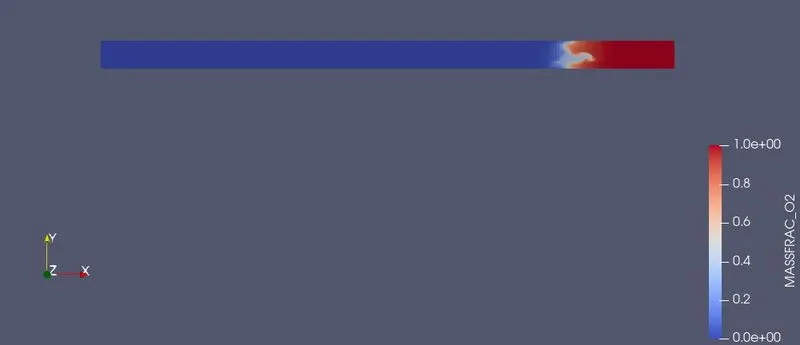
the pressure in the high pressure region is 6 bar and the pressure in the low pressure region is atmospheric pressure. here in the high pressure region i have taken N2 gas and in the low pressure region i have taken the O2 gas to see how they are mixed.

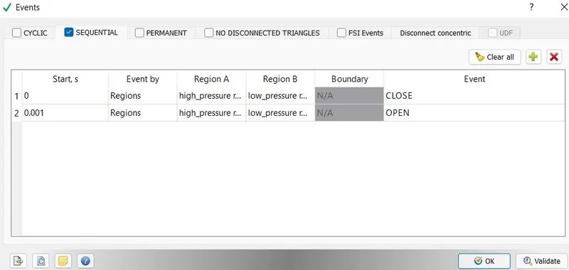
events- when two regions are in contact with each other with no boundaries in between them, then we use events. events create the triangles in between the two regions called disconnect triangles. in the below figure it is showing that at the start of time, the high pressure region and low pressure region are closes with each other. after the time 0.001 seconds, both regions should get open out that is the diaphrragm gets reptures in the shock tube.

boundary conditions:

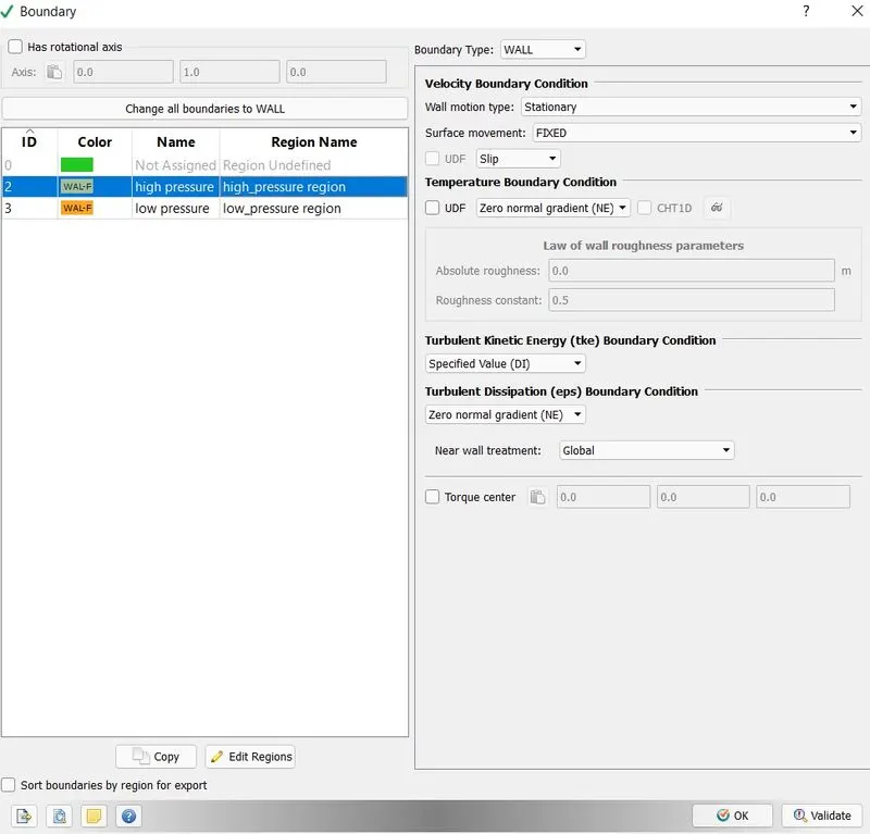
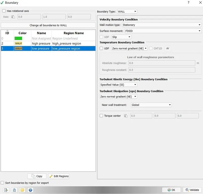
boundary-

• high pressure-

• low pressure-

physical models:

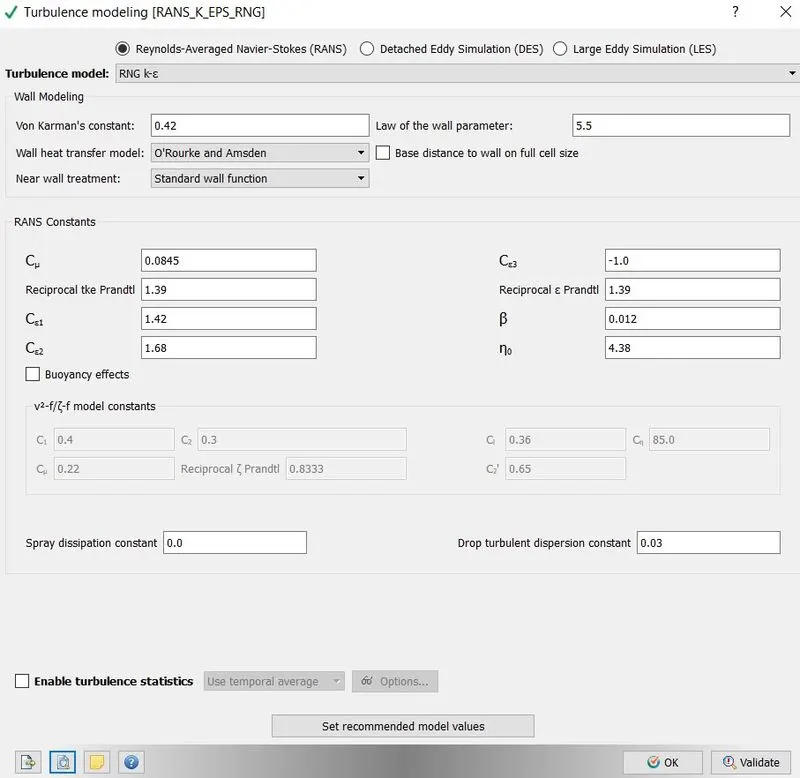
turbulence modelling-

grid control:

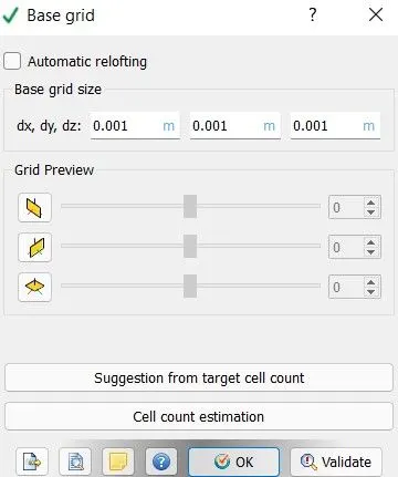
base grid-

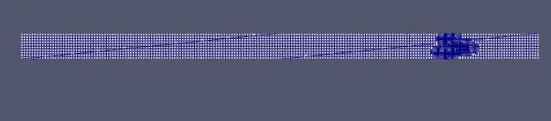
adaptive mesh refinement-

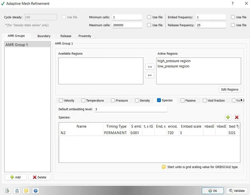
adaptive mesh refinement option is used to refine the mesh in the areas where the N2 is fluctuates more than the sub grid criteria. here i have taken the primitive variable is species. the sub grid criteria is also calles SGS parameter. the maximum embedding layers means the number of layers of cells that can be refined during the fluctuations of N2 to visualize clearly.

output/post-processing:

post variable selection-

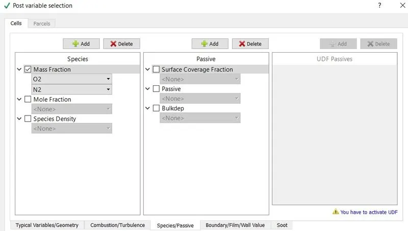
by selecting the different primitive variables in the post variable selection. we can see the contours of the variables in the paraview.

output-

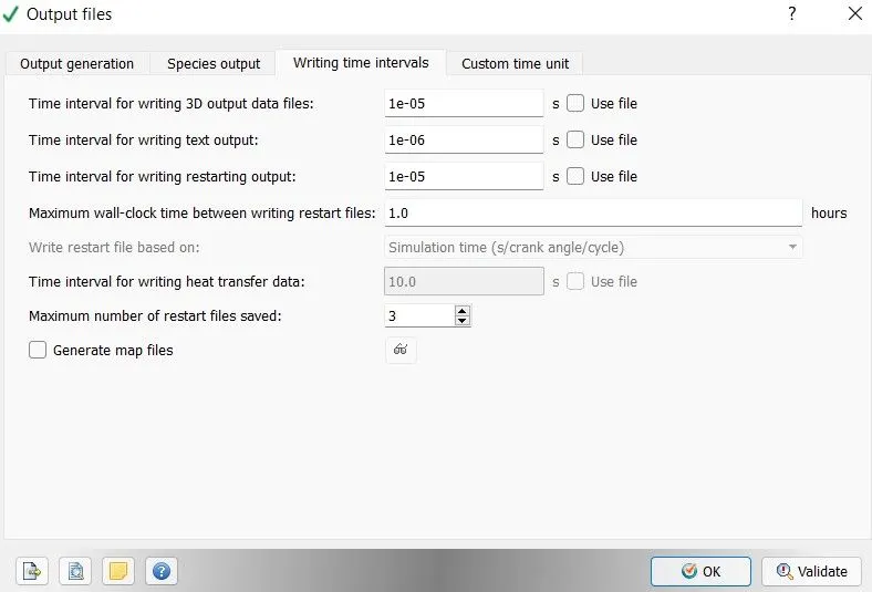
solution:

now export all the input files in a folder. so from this we can see that converge is used to create the input files for the simulation. now insert the two application files from the converge folder to the folder where i have exported all the input files.

for the simulation i have used cygwin64 terminal. in cygwin termpinal open the folder where you have pasted all the input and application files.

now for the simulation write mpiexec.exe -n 4 converge.exe restricted and click enter. here 4 represents the number of processors used at a time.

post processing of results:

for this copy post convert application from converge folder to output folder which is generated in the input files folder. we are doing this because we are goingto convert all the output files into a vtk file which can be easily read by paraview software. toconvert the files we have to use post conver application as shown in the figure. there we can see the results that are obtained. now in cygwin open the output folder and write mpiexec.exe -n 4 post_convert.exe and click enter. now the below figure will appear

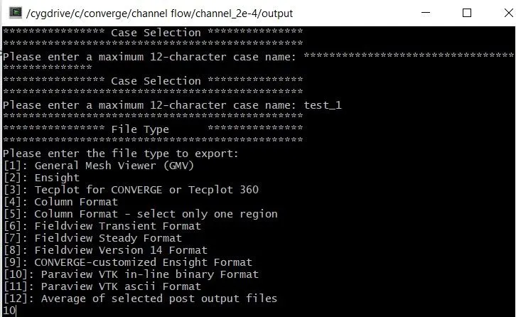
after naming the case and choosing 10, hit enter. now click yes for boundary output surface. now all the output files will appear and then write 'all' to convert all the output files. now select 'all' at cell variable selection menu. now all the files gets converted into paraview vtk files.

now open paraview. in paraview, open file and select case name .. vtm file which is present in the output files. finally we see the geometry in the paraview. now choose slice tool to select the axis along which all the primitive variables are same. as we know that, along z axis the primitive varibles are equal. so select axis and click apply.

grid-

final grid after AMR-

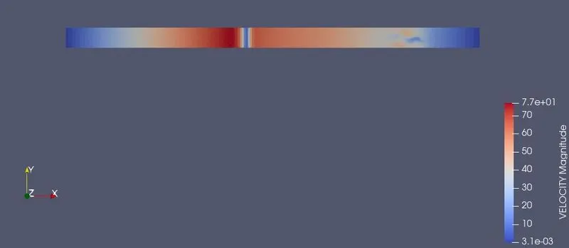
velocity contour-

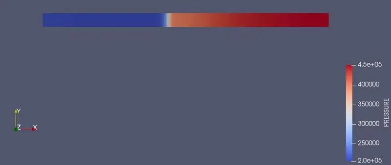
pressure contour-

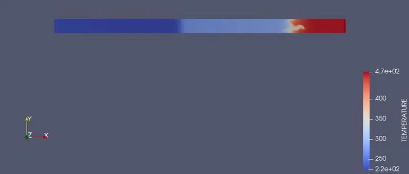
temperature contour-

N2 mass fraction contour-

O2 mass fraction-

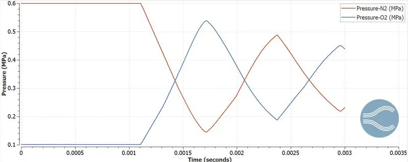
pressure contour-

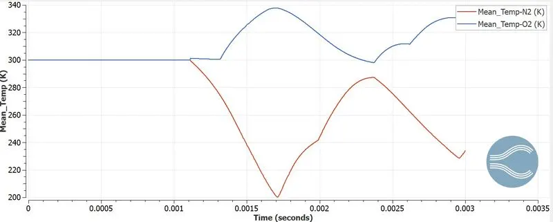
temperature contour-

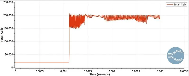
total cell count-

conclusion:

• with the expansion of high pressure region, the pressure of the N2 gets reduced and the with the compreesion of low pressure region because of the high pressure region, the pressure of O2 gets increased. from yhe plot we can say that the pressure of N2 and O2 are inversly proportional.
• the temperature of the N2 gets reduced because of the expansion of the N2 and the temperature of the O2 gets increased because of the compression of O2 gas.
• the total cell count keeps on varied because of the adpative mesh refinement.