Week 8 - Simulation of a backward facing step in OpenFOAM
AIM:
Simulation of backward facing step in openfoam.
Objectives:
Case 1 - to Simulate the flow without using any grading factor (i.e., GF = 1)
Case 2 - to Simulate the flow with grading factor of 0.2. The cells should be finer near the walls (includig the step wall).
theory:
here we are considering the flow as incomressble laminar viscus flow and we are trying to do how this flow happens in backward facing step geometry. so we are going to use icofoam solver in the openfoam for laminar incompressible flow .
initially we are going to make the geometry using blockMesh and we are going to make the geomtry as small cells. so that we we can easily apply finite volume method to the cell to get the accurate values of primitive varibales at each cell.
the given backward facing step geometry is
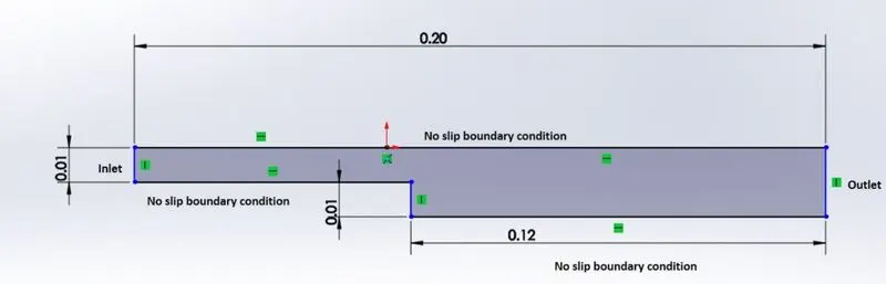
- Number of cells along the x direction (longer dimension) = 200
- Number of cells along the longer y direction = 20;
now we are going to make the geometry into five blocks

here we are majorly considering the geometry is in 2d with minimum thickness along z axis with 0.001mm.
firstly in the blockmesh we are going to denote vertices , the below figure shows the vertices of the geometry
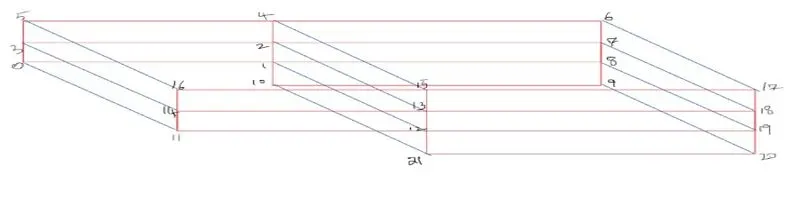
after that we going to denote blocks, here we have 5 blocks now we are going to cut the block into cells. finally the below file represents the blockmeshdict file which consists of blockmesh.
case 1:
FoamFile
{
    version     2.0;
    format      ascii;
    class       dictionary;
    object      blockMeshDict;
}
// * * * * * * * * * * * * * * * * * * * * * * * * * * * * * * * * * * * * * //

convertToMeters 1;

vertices
(
    (0 0 0)
    (0.08 0 0)
    (0.08 0.005 0)
    (0 0.005 0)
    (0.08 0.01 0)
    (0 0.01 0)
    (0.2 0.01 0)
    (0.2 0.005 0)
    (0.2 0 0)
    (0.2 -0.01 0)
    (0.08 -0.01 0)

    (0 0 0.001)
    (0.08 0 0.001)
    (0.08 0.005 0.001)
    (0 0.005 0.001)
    (0.08 0.01 0.001)
    (0 0.01 0.001)
    (0.2 0.01 0.001)
    (0.2 0.005 0.001)
    (0.2 0 0.001)
    (0.2 -0.01 0.001)
    (0.08 -0.01 0.001)
);

blocks
(
    hex (0 1 2 3 11 12 13 14) (80 5 1) simpleGrading (1 1 1)
    hex (3 2 4 5 14 13 15 16) (80 5 1) simpleGrading (1 1 1)
    hex (2 7 6 4 13 18 17 15) (120 5 1) simpleGrading (1 1 1)
    hex (1 8 7 2 12 19 18 13) (120 5 1) simpleGrading (1 1 1)
    hex (10 9 8 1 21 20 19 12) (120 10 1) simpleGrading (1 1 1)
);

edges
(
);

boundary
(
    inlet
    {
        type patch;
        faces
        (
            (16 5 3 14)
            (14 3 0 11)
        );
    }
    outlet
    {
        type patch;
        faces
        (
            (7 6 17 18)
            (8 7 18 19)
            (9 8 19 20)
        );
    }
    noSlipWalls
    {
        type wall;
        faces
        (
            (10 9 20 21)
            (5 16 15 4)
            (4 15 17 6)
            (10 21 12 1)
            (0 1 12 11)
        );
    }
    frontAndBack
      {
          type empty;
          faces
         (
             (14 13 15 16)
             (11 12 13 14)
             (13 18 17 15)
             (12 19 18 13)
             (21 20 19 12)
             (3 5 4 2)
             (0 3 2 1)
             (2 4 6 7)
             (1 2 7 8)
             (10 1 8 9)
        );
     }
);

mergePatchPairs
(
);

// ************************************************************************* //
after denoting blocks we are going to choose boundaries that through which flow goes in and out and what are the walls are there in the geomtry we going to denote them. patches are represented to inlet and outlet boundaries where as walls are denoted to remaining boundaries.
next we are going to give initial values for primitive variables. here we have used two primitive variables that are velocity and pressure. the below file represents the initial values of velocity.
FoamFile
{
    version     2.0;
    format      ascii;
    class       volVectorField;
    object      U;
}
// * * * * * * * * * * * * * * * * * * * * * * * * * * * * * * * * * * * * * //

dimensions      [0 1 -1 0 0 0 0];

internalField   uniform (0 0 0);

boundaryField
{
     inlet
    {
        type            fixedValue;
        value           uniform (1 0 0);
    }

    outlet
    {
        type            zeroGradient;
    }

    noSlipWalls
    {
        type            noSlip;
    }

    frontAndBack
    {
        type            empty;
    }

}

// ************************************************************************* //
here we have used inlet velocity as 1m/s. at let we have used zero gradient which represents the neumann boundary condition,from which we can find the outlet velocity. the top, bottem and side boundary are given as no slip. which means the velocity at that positions are zeros. we represented front and back as empty because we are manily consderng the geometry as 2dimensional and the flow also as 2dimensional.
the below file represents the pressure
FoamFile
{
    version     2.0;
    format      ascii;
    class       volScalarField;
    object      p;
}
// * * * * * * * * * * * * * * * * * * * * * * * * * * * * * * * * * * * * * //

dimensions      [0 2 -2 0 0 0 0];

internalField   uniform 0;

boundaryField
{
    inlet
    {
        type            zeroGradient;
    }

    outlet
    {
        type            fixedValue;
        value           uniform 0;
    }

    noSlipWalls
    {
        type            zeroGradient;
    }

    frontAndBack
    {
        type            empty;
    }
}

// ************************************************************************* //
here we have taken the pressure as zero at inlet and at outlet.
after that we are going to chane the modifications in controldict file which represnts the start and end time of the flow and the dt value. the value of dt value is taken from courant number. the below file represents the controldict file
FoamFile
{
    version     2.0;
    format      ascii;
    class       dictionary;
    location    "system";
    object      controlDict;
}
// * * * * * * * * * * * * * * * * * * * * * * * * * * * * * * * * * * * * * //

application     icoFoam;

startFrom       startTime;

startTime       0;

stopAt          endTime;

endTime         0.5;

deltaT          0.00025;

writeControl    timeStep;

writeInterval   20;

purgeWrite      0;

writeFormat     ascii;

writePrecision  6;

writeCompression off;

timeFormat      general;

timePrecision   6;

runTimeModifiable true;


// ************************************************************************* //
Results:
after using of icofoam solver we are going to get the values of primitive variables at at each cell and we can see how flow moves along the geometry in the parafoam
the below figure represnts the geomtery with mesh of grading factor 1

the below figure shows the velocity with whcih the fow moves along the geometry
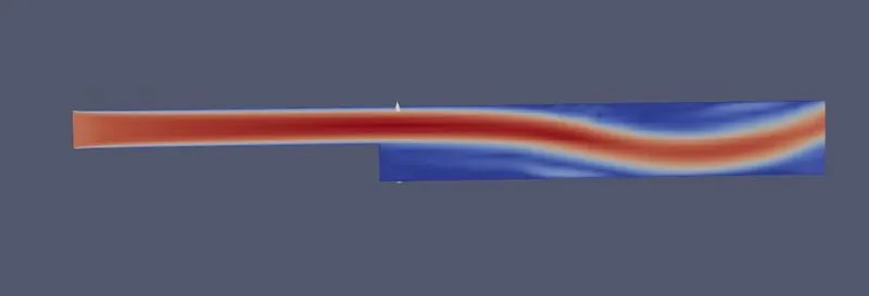
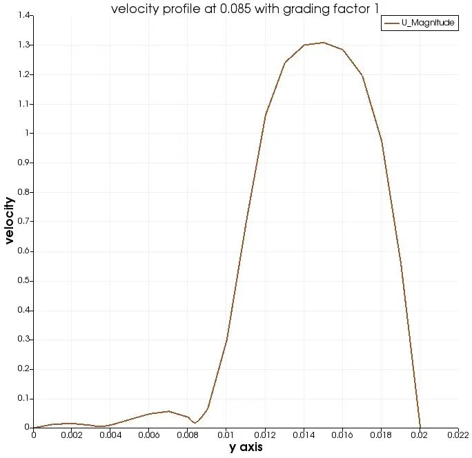
the blue line reprensts the no slip walls with velocity zero. the below figure represents the velocity profile at 0.085m. with grading factor 1.
case 2:
here we are going to use grading factor 0.2.
grading factor means it is the ratio of size of end cell to the size of starting cell. if the size of the cell is smaller, then by using of finite volume method, to get primitive variables we get accurate results as we are taking average values at the centre of the cell.
by taking grading factor 0.2 we can modify the blockmeshdict file. the below file represents the blockmeshdict file with grading factor 0.2
FoamFile
{
    version     2.0;
    format      ascii;
    class       dictionary;
    object      blockMeshDict;
}
// * * * * * * * * * * * * * * * * * * * * * * * * * * * * * * * * * * * * * //

convertToMeters 1;

vertices
(
    (0 0 0)
    (0.08 0 0)
    (0.08 0.005 0)
    (0 0.005 0)
    (0.08 0.01 0)
    (0 0.01 0)
    (0.2 0.01 0)
    (0.2 0.005 0)
    (0.2 0 0)
    (0.2 -0.01 0)
    (0.08 -0.01 0)

    (0 0 0.001)
    (0.08 0 0.001)
    (0.08 0.005 0.001)
    (0 0.005 0.001)
    (0.08 0.01 0.001)
    (0 0.01 0.001)
    (0.2 0.01 0.001)
    (0.2 0.005 0.001)
    (0.2 0 0.001)
    (0.2 -0.01 0.001)
    (0.08 -0.01 0.001)
);

blocks
(
    hex (0 1 2 3 11 12 13 14) (80 5 1) simpleGrading (0.2 5 1)
    hex (3 2 4 5 14 13 15 16) (80 5 1) simpleGrading (0.2 0.2 1)
    hex (2 7 6 4 13 18 17 15) (120 5 1) simpleGrading (5 0.2 1)
    hex (1 8 7 2 12 19 18 13) (120 5 1) simpleGrading (5 5 1)
    hex (10 9 8 1 21 20 19 12) (120 10 1) simpleGrading (5 5 1)
);

edges
(
);

boundary
(
    inlet
    {
        type patch;
        faces
        (
            (16 5 3 14)
            (14 3 0 11)
        );
    }
    outlet
    {
        type patch;
        faces
        (
            (7 6 17 18)
            (8 7 18 19)
            (9 8 19 20)
        );
    }
    noSlipWalls
    {
        type wall;
        faces
        (
            (10 9 20 21)
            (5 16 15 4)
            (4 15 17 6)
            (10 21 12 1)
            (0 1 12 11)
        );
    }
    frontAndBack
      {
          type empty;
          faces
         (
             (14 13 15 16)
             (11 12 13 14)
             (13 18 17 15)
             (12 19 18 13)
             (21 20 19 12)
             (3 5 4 2)
             (0 3 2 1)
             (2 4 6 7)
             (1 2 7 8)
             (10 1 8 9)
        );
     }
);

mergePatchPairs
(
);
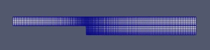
result:
the below figure represents final mesh with grading factor 0.2
the below figure reprents the velocity with which the flow moves along the geometry

the below figure represents the velocity profile at 0.085m. with grading factor 0.2
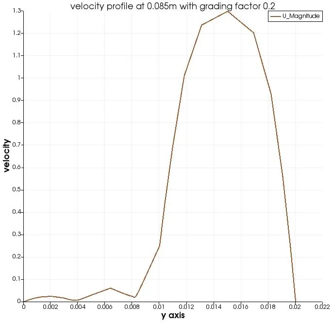
- the maximum velocity in y axis at 0.01498m with grading factor 1.
- the maximum velocity in y axis at 0.0150m with grading factor 0.2