Week 4 - CHT Analysis on Exhaust port

AIM:

CHT Analysis on Exhaust port

objectives:

1. Give a brief description of why and where a CHT analysis is used.
2. Maintain the y+ value according to the turbulence model and justify the results.
3. Calculate the wall/surface heat transfer coefficient on the internal solid surface & show the velocity & temperature contours in appropriate areas.
4. How would you verify if the HTC predictions from the simulations are right? On what factors does the accuracy of the prediction depend on?

1.brief description of why and where a CHT analysis is used:

Conjugate heat transfer corresponds with the combination of heat transfer in solids and heat transfer in fluids. In solids, conduction often dominates whereas in fluids, convection usually dominates. Conjugate heat transfer is observed in many situations. For example, heat sinks are optimized to combine heat transfer by conduction in the heat sink with the convection in the surrounding fluid. The temperature field and the heat flux are continuous at the fluid/solid interface. However, the temperature field can rapidly vary in a fluid in motion: close to the solid, the fluid temperature is close to the solid temperature, and far from the interface, the fluid temperature is close to the inlet or ambient fluid temperature. The distance where the fluid temperature varies from the solid temperature to the fluid bulk temperature is called the thermal boundary layer. The thermal boundary layer size and the momentum boundary layer relative size is reflected by the Prandtl number.

Prandtl number = `(C_p . mu)/K`

where `C_p` is heat capacity at constant pressure (SI unit: J/kg.K)

`mu`is the absolute visosity (SI unit: NS/m^2)

K is the thermal conductivity (SI unit: W/m.k)

for the Prandtl number to equal 1, thermal and momentum boundary layer thicknesses need to be the same. A thicker momentum layer would result in a Prandtl number larger than 1. Conversely, a Prandtl number smaller than 1 would indicate that the momentum boundary layer is thinner than the thermal boundary layer. The Prandtl number for air at atmospheric pressure and at 20°C is 0.7. That is because for air, the momentum and thermal boundary layer have similar size, while the momentum boundary layer is slightly thinner than the thermal boundary layer. higher the thermal boundary layer, there will br higher the heat transfer from fluid to solid.

2. y+ value:

y+ is a non-dimensional distance. It is important in turbulence modelling to determine the proper size of the cells near domain walls to check if the mesh is fine enough to catch the boundary layer near the walls. the value of y+ is different for different turbulence models. for k-epsilon standard turbulance model the y+ value id ranging from 30 to 300, for k-omega SST model the y+ value is ranging from 0 to 5.

to determine the size of the cell at the boundary, that is first layer thickness we have to use below formulae

Firstly, we should calculate the Reynolds number for our model based on the characteristic scales of our geometry such that:

`Re = (rho.U.L)/mu`,

where `rho` and `mu` are the fluid density and viscosity respectively

`U` is the freestream velocity

L is the characteristic length (e.g. pipe diameter, body length, etc.).

The definition of the y+ value is such that:

`Y+ = (rho. Ut.∆y1)/μ``→ ∆y1=(Y+.μ)/(rho.Ut)`

the frictional velocity, Ut is defined as:

`Ut = √(τ_w/ρ)`

The wall shear stress, `tau_w` can be calculated from skin friction coefficient, `Cf`, such that:

`tau_w = 1/2.Cf.rho.U^2`

for an external flow, the Cf value is defined as:

`Cf = 0.058 * Re^-0.2`

by using the above formulae we can calculate the first layer thickness. here we are taking air as fluid and we are going to take the default values of air from ansys fluent. i am going to use k-epsilon standard turbulent model for the simulation. so i can take the values of y+ in between 30 to 300.

3. Calculate the wall/surface heat transfer coefficient on the internal solid surface & show the velocity & temperature contours in appropriate areas:

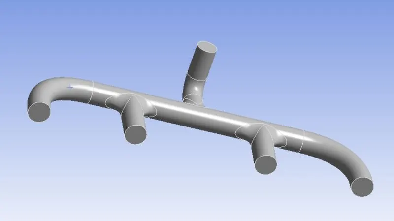
geoemtry of exhaust port:

solid part-

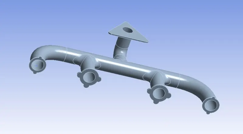
fluid volume-

final geometry-

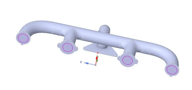
there are four inlets and one outlet in the exhaust port.

baseline mesh:

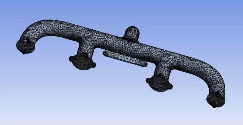
this is the mesh generated from the geometry by using default values from the mesh. the four inlets were named as inlets and the one outlet is named as outlet and the outer surface of exhaust port is named as ourt wall convection. i have named it because the mode of heat transfer from outer surface to air around the exhaust port is convection. so i have bamed the outer surface of exhaust port as outer wall convction.

setup:

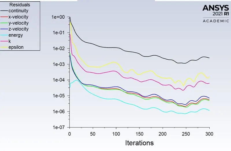
here the inlet velocity of fluid is 5m/s and the temperatures of inlet fluid is 700k. the pressure based solver is used with steady state condition. k epsilon standard model is used here and the convective heat transfer coefficent at outer wall convection value is 20 w/m^2.k . make the temperature contour at the outer wall convection. run the simulation for 300 iterations.

solution:

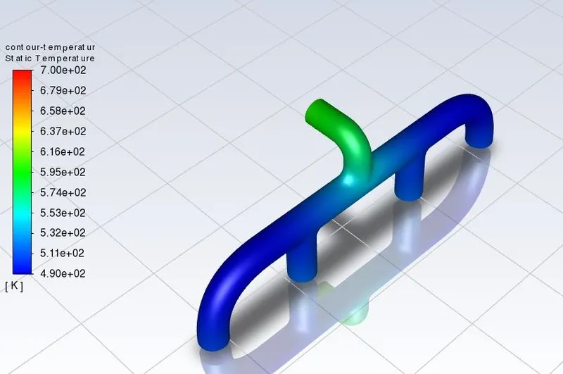
final temperature contour-

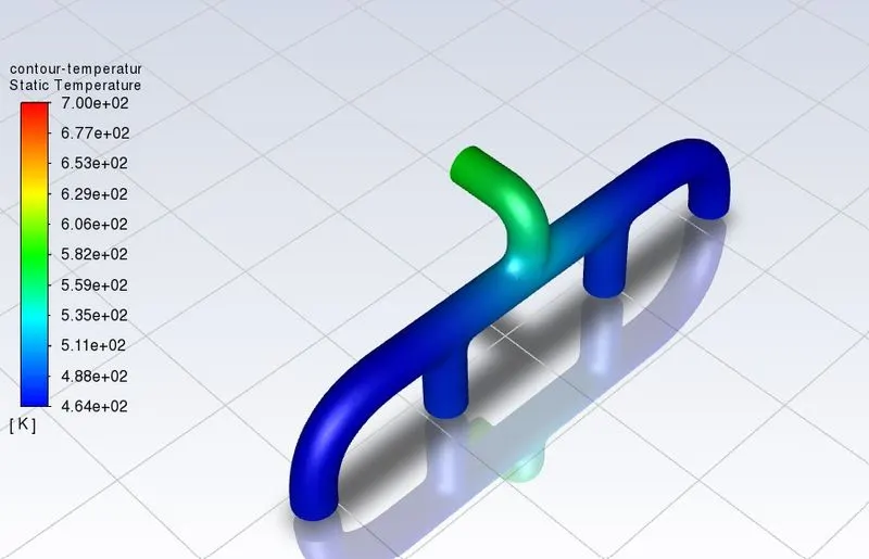
here from the contour we are seeing that the temperature at oulet port is higher than the temperature of the inlet ports. because as we know that the mass flow rare is same at every crosee section of the exhaust port that is mass flow rate at inlet ports is equal to mass flow rate at outlet port. here the area of the all inlet and outlet ports is same with diamter of 166 mm.

mass flow rate at inlet ports = mas flow rate at outlet port

a1.v1 + a2.v2 + a3.v3 + a4.v4 = a5.v5

where a1,a2,a3,a4,a5 are areas of inlet and outlet of exhaust port and v1,v2,v3,v4,v5 are the velocitites of fluid in the exhaust port at inlets and outlet port.

as the areas are almost equal then we can write the above equation as

v1+v2+v3+v4 = v5.

from this we can say that the exhaust gases moves out with high velocity. as we know that the temperature is a function of velocity, so temperature at outlet is greater than temperature at inlets.

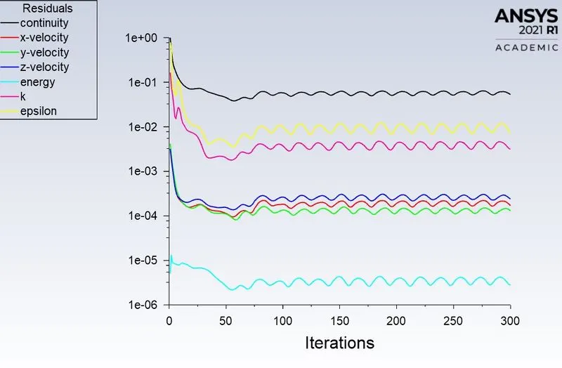
residuals plot-

results:

velocity streamlines-

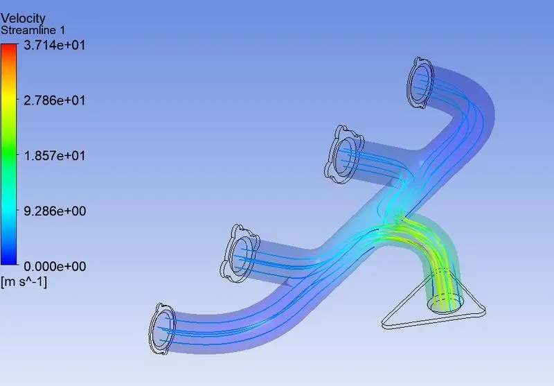
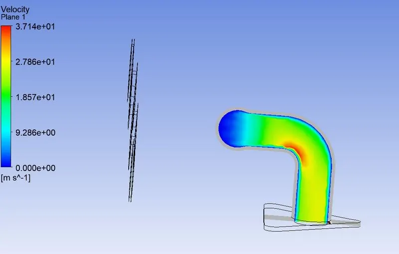
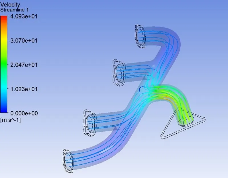
as we discussed above , the velocity at the outer port is higher which is shown in the above figure.

velocity plane at the outer port-

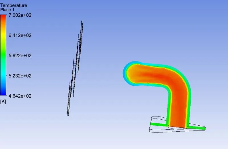
temperature plane at outer port-

the exhaust port with refined mesh:

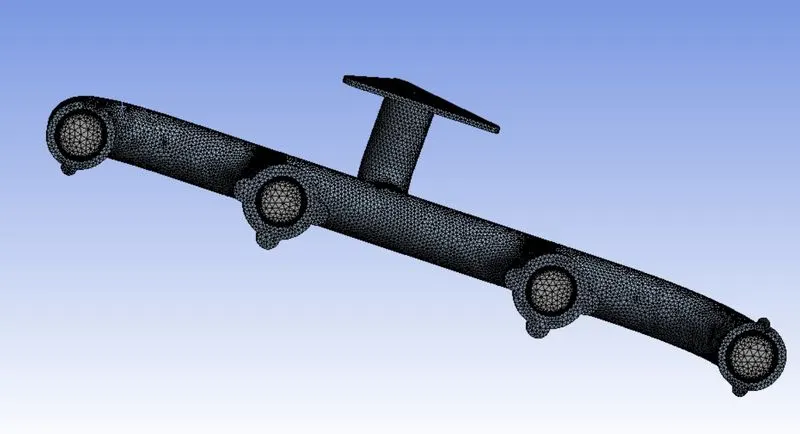
here the eklement size of the solid body is 15mm and the y+ value is taken here is 30 and the first layer thickness obtained is 1.68027007449014E-03. the total number of elements produced is 495926.

solution:

final temperature contour-

residuals plot-

surface heat transfer coefficent plot-

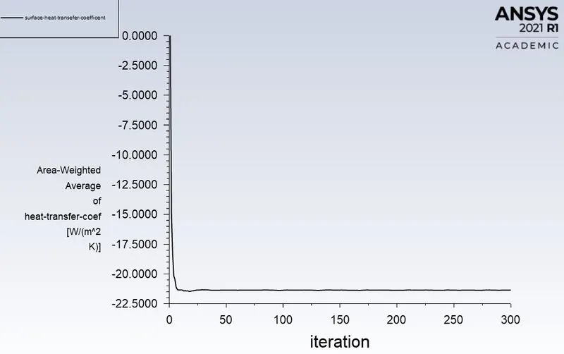
it is the convective heat transfer coefficent of the the fluid in exhaust port. the magnitude surface heat transfer coefficent is 21.357019 w/m^2.k

here the heattransfer coefficent is shown in negative values because of temperature difference due to heat transfer.

result:

velocity streamlines-

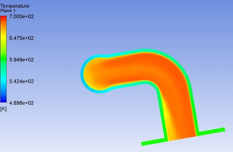
temperature plane at the outer port-

velocity plane at the outer port-

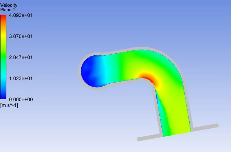
we can clearly visualize the increase of velocity at the bent portion of outlet port. this is because of refining of mesh and creating of inflation layers at the wall boundary.

4.How would you verify if the HTC predictions from the simulations are right? On what factors does the accuracy of the prediction depend on?

the formula for nusselt number is ratio of convective heat transfer to conductive heat transfer

nasselt number = `(h.L)/K`

where h is the convective heat transfer coefficent

L is the charecterstic length

K is the conductive heat transfer coefficent

in the above problem charecterstic length is diameter of the exhaust port. we know that reynolds number is a function of charecterstic length. so we can conclude here that nusselt number is a finctin of reynolds numer.

reynold number = `(rho.v.L)/mu`

where v is the velocity of flow

`mu`is the absolute viscosity

`rho`is the density of fluid in the exhaust port.

from the above conclusion and the above two formulae we can say that h is directly proportional to velocity, that is heat transfer coefficent(htc) is directly proportional to velocity of fluid inside the exhaust port.

in the above figures we have clearly seen the velocity of fluid in the outlet port using refined elemet size compared to baseline elements. so we can also say that heat transfer coefficent can be clearly visualized using the refined element size.

the factory consider for the accuracy of predictions are refining of element size and providing of inflation layers at the boundaries of the exhaust fluid flow.