Week 5.1 - Mid term project - Solving the steady and unsteady 2D heat conduction problem
AIM :
solving the steady and unsteady 2D heat conduction problem.
Governing equation:
`(∂ T)/(∂ t) + α((∂^2 T)/(∂x^2 ) + (∂^2 T)/(∂y^2 )) = 0`
where α is constant thermal diffusivity.
here constant α = 2*1e-4 (units : `m^2/s`)
Theory:
here we have 2D plate with with very low thickness. At each side of plate there is each temperature is present. in the problem
T_left = 400
T_right = 800
T_bottem = 900
T_top = 600
with this input temperature, we are going to find out how the heat getting flows inside the plate from all sides and how the temperature gets distributed in the plate surface. for this we are going to use two forms
1. explicit form : in this form we know all the values in the right hand side of the equation. we are going to find out only value that is left hand side of the equation. for this we mostly won't use iteration techniques. iteration techniqus are used to solve complex equations with more unknowns. we are going to write the above governing equation in explicit form.
`(T(i,j)^(n+1)-T(i,j)^n)/dt = -α( (T(i+1,j)^n-2T(i,j)^n+T(i-1,j)^n)/(dx^2 ) + (T(i,j+1)^n-2T(i,j)^n+T(i,j-1)^n)/(dy^2 ))`
here we know the temperature with n'th time step. it means temperature at initial condition. temperature with n+1 time step means we are going to find the temperture after some time dt. from this we are we are going to find out temperature at every node after some time t.
2. implicit form : in this form we don't know the values in both left hand side and right hand side. so many equations are obtained here. so to solve them we use iteration techniques here. we are going to write the above governing equation in explicit form.
`(T(i,j)^(n+1)-T(i,j)^n)/dt = -α( (T(i+1,j)^(n+1)-2T(i,j)^(n+1)+T(i-1,j)^(n+1))/(dx^2 ) + (T(i,j+1)^(n+1)-2T(i,j)^(n+1)+T(i,j-1)^(n+1))/(dy^2 ))`
we are taking dx = dy.
here the we are going to find out heat conducted during steady state and transient state.
Steady state 2D heat conduction:
steady state condition means the temperature depends on only the space but not time. we can solve this problem by using iteration techniques like jacobi iteration technique, gauss seidal iteration technique, Successive over relaxation method.
jacobi iteration technique:
`T(i,j)^(n+1)= (T(i-1,j)^n+T(i+1,j)^n+ T(i,j-1)^n+T(i,j+1)^n)/4`
gauss seidal iteration technique:
`T(i,j)^(n+1)= (T(i-1,j)^(n+1)+T(i+1,j)^n+T(i,j-1)^(n+1)+T(i,j+1)^n)/4`
successive over relaxation technique:
`T(i,j)^(n+1)=(1-β)T(i,j)^n+β((T(i-1,j)^(n+1)+T(i+1,j)^n+T(i,j-1)^(n+1)+T(i,j+1)^n)/4)`
here ' beta ' is relaxation parameter. Relaxation parameter is used to control the convergence of iteration process. the optimal values of relaxation parameters are 1.1,1.2 . if relaxation parameter is less than 1, we can call it as under relaxation parameter. if the relaxation parameter is greater than 1.2, we can call it as over ralaxation parameter. with uder and over relaxation parameters, it takes more time to get the steady state solution.
Main code:
clear all
close all
clc

%inputs
nx = 10;
ny = 10;
x = linspace(0,1,10);
y = linspace(0,1,10);
dx = x(2)-x(1);
dy = y(2)-y(1);

%temperatures
T = 300*ones(nx,ny);
T(:,1) = 400;
T(:,end) = 800;
T(1,:) = 600;
T(end,:) = 900;
Told = T;
tol = 1e-4;
error = 10;
iteration_solver = 3;
%jacobi method
if iteration_solver ==1
    jacobi_iter = 1;
    while (error>tol)
        for j = 2:ny-1
            for i = 2:nx-1
                T(i,j) = (Told(i-1,j)+Told(i+1,j)+Told(i,j-1)+Told(i,j+1))/4;
            end
        end
        error =max(max(abs(Told-T)));
        Told = T;
        jacobi_iter = jacobi_iter+1;
    end
        figure(1)
        contourf(x,y,T,'ShowText','ON')
        colorbar
        colormap(jet)
        xlabel('x axis')
        ylabel('y axis')
        title_text = sprintf('steady state jacobi iteration number = %d',jacobi_iter);
        title(title_text)
end

%gs method
if iteration_solver ==2
    gs_iter = 1;
    while (error>tol)
        for j = 2:ny-1
            for i = 2:nx-1
                T(i,j) = (T(i-1,j)+Told(i+1,j)+T(i,j-1)+Told(i,j+1))/4;
            end
        end
        error = max(max(abs(Told-T)));
        Told = T;
        gs_iter = gs_iter+1;
    end
        figure(2)
        contourf(x,y,T,'ShowText','ON')
        colorbar
        colormap(jet)
        xlabel('x axis')
        ylabel('y axis')
        title_text = sprintf('steady state gs iteration number = %d',gs_iter);
        title(title_text)
end

%SOR method
beta = 1.2;
relaxation_parameter = 1.2;
if iteration_solver ==3
    SOR_iter = 1;
    while (error>tol)
        for j = 2:ny-1
            for i = 2:nx-1
                T(i,j) = (1-beta)*(Told(i,j)) +(beta*((T(i-1,j)+Told(i+1,j)+T(i,j-1)+Told(i,j+1))/4));
            end
        end
        error = max(max(abs(Told-T)));
        Told = T;
        SOR_iter = SOR_iter+1;
    end
        figure(3)
        contourf(x,y,T,'ShowText','ON')
        colorbar
        colormap(jet)
        xlabel('x axis')
        ylabel('y axis')
        title_text = sprintf('steady state SOR iteration number = %d',SOR_iter);
        title(title_text)
end
output of the code:
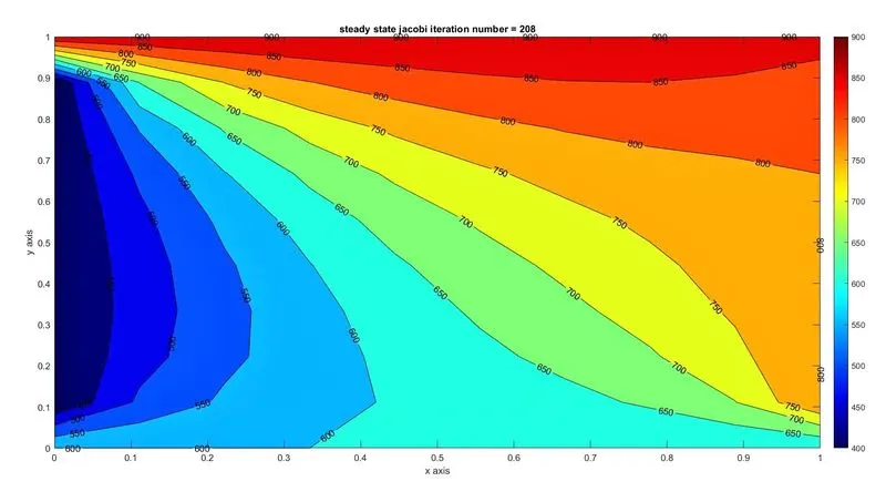
jacobi plot-
figure(1)
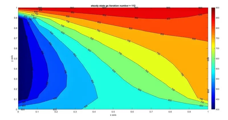
gauss seidal plot:
figure(2)
SOR plot-
figure(3)
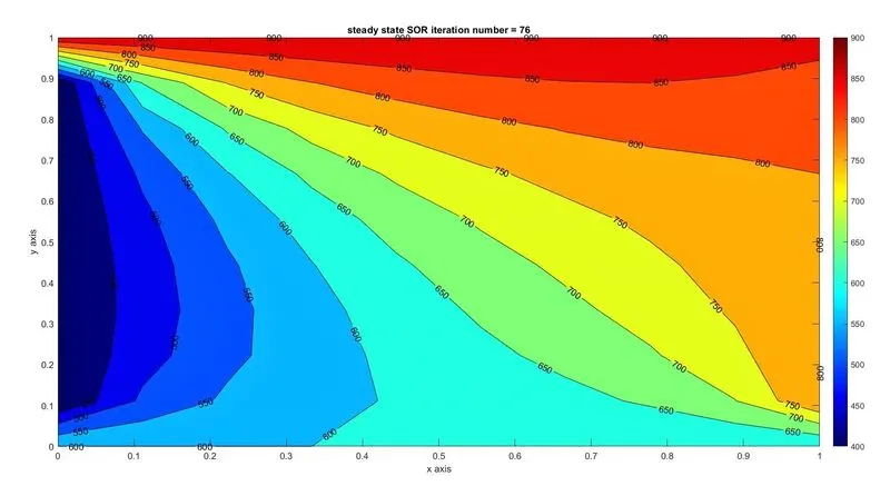
by seeing the plots we can say that the solution reached to steady state condition. to reach the steady state jacobi took 208 iterations, gauss seidal took 112 iterations where as SOR took 76 iterations. less number of iteration means the solution gets converges fastly to steady state.
from this we coclude that SOR technique is better than gauss seidal and jacobi iteration techniques in the steady state 2d heat conduction problem.
Transient state 2D heat conduction:
Transient state condition means the temperature depends on both space and time. here we can use either explicit or implicit form to obtain the solution.
- transient explicit form: here we directly solve problem without using iterations techniques beacuse we have only one unknown in the below equation.
`T(i,j)^(n+1)=T(i,j)^n+CFL1*(T(i+1,j)^n-2T(i,j)^n+T(i-1,j)^n )+CFL2*(T(i,j+1)^n-2T(i,j)^n+T(i,j-1)^n)`
CFL indicates Courant number. the Courant number is used to obtain the time steps requied to in transient simlation problem to get to the steady state position. the CFL number
`CFL1=α dt/(dx^2 )` `CFL2=α dt/(dy^2 )`
for 2D heat conduction problem,
`CFL=α dt/(dx^2 )+α dt/(dy^2 ) ≤0.5`
main code:
clear all
close all
clc

%inputs
nx = 10;
ny = 10;
x = linspace(0,1,10);
y = linspace(0,1,10);
dx = x(2)-x(1);
dy = y(2)-y(1);

%temperatures
T = 300*ones(nx,ny);
T(:,1) = 400;
T(:,end) = 800;
T(1,:) = 600;
T(end,:) = 900;
Told = T;
%CFL1 = alfa*dt/dx^2  CFL2 = alfa*dt/dy^2
alfa = 2*1e-4;
t = 22500;
dt = 15;
nt = t/dt;
CFL1 = alfa*dt/dx^2;
CFL2 = alfa*dt/dy^2;
CFL = CFL1+CFL2;
%time loop
iter = 1;
for k = 1:nt
    %space loop
    for j = 2:ny-1
        for i = 2:nx-1
            T(i,j) = Told(i,j)+(CFL1*(Told(i-1,j)-2*Told(i,j)+Told(i+1,j)))+(CFL2*(Told(i,j-1)-2*Told(i,j)+Told(i,j+1)));
        end
    end
    Told = T;
    iter = iter+1;
end
    figure(5)
    contourf(x,y,T,'ShowText','ON');
    colorbar;
    colormap(jet);
    xlabel('x axis');
    ylabel('y axis');
    title_text = sprintf('transient explicit iteration number = %d and time = %f and CFL = %f',iter,t,CFL);
    title(title_text);
output of code:
figure(4)
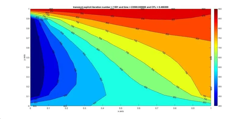
figure(5)
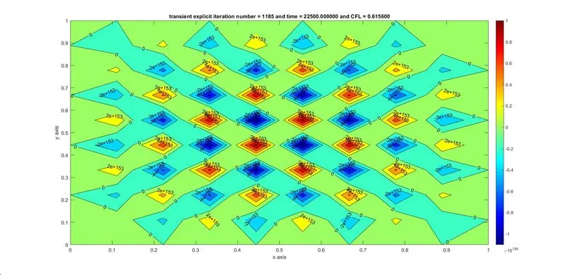
figure (5) shows that solution reached to steady state position. but figure (6) shows that solution gets diverged,because in the figure(5) we have taken CFL number is 0.48 which is less than 0.5. but in figure(6) we have taken CFL number as 0.615 which is grater than 0.5.
so from this we can conclude that in solving transient explicit problem the CFL number should always be less than or equal to 0.5
- Transient implicit form: here we are going to use iteration techniques as we know that implicit form has more number of unknowns with more equations.
jacobi iteration technique:
`T(i,j)^(n+1)=term1*Tprev(i,j)^n+term2*(T(i-1,j)^n+T(i+1,j)^n )+term3*(T(i,j-1)^n+T(i,j+1)^n)`
gauss seidal technique:
`T(i,j)^(n+1)=term1*Tprev(i,j)^n+term2*(T(i-1,j)^(n+1)+T(i+1,j)^n )+term3*(T(i,j-1)^(n+1)+T(i,j+1)^n)`
successive over relaxation technique:(SOR)
`T(i,j)^(n+1)=(1-β)T(i,j)^n+β(term1*Tprev(i,j)^n+term2*(T(i-1,j)^(n+1)+T(i+1,j)^n )+term3*(T(i,j-1)^(n+1)+T(i,j+1)^n))`
where as Tprev indicates the temperature of previous time step. 'beta' relaxation parameter.
main code:
close all
clear all
clc

%inputs
nx = 10;
ny = 10;
x = linspace(0,1,10);
y = linspace(0,1,10);
dx = x(2)-x(1);
dy = y(2)-y(1);

%temperatures
T = 300*ones(nx,ny);
T(:,1) = 400;
T(:,end) = 800;
T(1,:) = 600;
T(end,:) = 900;
Told = T;
%CFL1 = alfa*dt/dx^2  CFL2 = alfa*dt/dy^2
alfa = 2*1e-4;
t = 22500;
dt = 15;
nt = t/dt;
CFL1 = alfa*dt/dx^2;
CFL2 = alfa*dt/dy^2;
CFL = CFL1+CFL2;
term1 = 1/(1+(2*CFL1)+(2*CFL2));
term2 = CFL1*term1;
term3 = CFL2*term1;
tol = 1e-4;
error = 10;
Tprev = T;
iteration_solver = 3;

%jacobi iteration
jacobi_iter = 1;
if iteration_solver ==1
for k = 1:nt
        error = 1;
        while(error>tol)
            for i = 2:nx-1
                for j = 2:ny-1
                    T(i,j) = (term1*Tprev(i,j))+(term2*(Told(i-1,j)+Told(i+1,j)))+(term3*(Told(i,j-1)+Told(i,j+1)));
                end
            end
            error = max(max(abs(Told-T)));
            Told = T;
     jacobi_iter = jacobi_iter+1;
        end
    Tprev = T;
end
    figure(6)
    contourf(x,y,T,'ShowText','ON')
    colorbar
    colormap(jet)
    xlabel('x axis')
    ylabel('y axis')
    title_text = sprintf('Transient implicit jacobi iteration number = %d and time = %f and CFL = %f',jacobi_iter,t,CFL);
    title(title_text)
end


%gs iteration
 gs_iter = 1;
 if iteration_solver ==2
for k = 1:nt
      error = 1;
        while(error>tol)
            for j = 2:ny-1
                for i = 2:nx-1
                    T(i,j) = (term1*Tprev(i,j))+(term2*(T(i-1,j)+Told(i+1,j)))+(term3*(T(i,j-1)+Told(i,j+1)));
                end
            end
            error = max(max(abs(T-Told)));
            Told = T;
            gs_iter = gs_iter+1;
        end

        Tprev = T;
end
        figure(7)
        contourf(x,y,T,'ShowText','ON')
        colorbar
        colormap(jet)
        xlabel('x axis')
        ylabel('y axis')
        title_text = sprintf('Transient implicit gs iteration number = %d and time = %f and CFL number = %f',gs_iter,t,CFL);
        title(title_text)
 end


%SOR method
beta = 1.1;
SOR_iter = 1;
if iteration_solver ==3
for k = 1:nt
      error = 1;
    while (error>tol)
        for i = 2:nx-1
            for j = 2:ny-1
                T(i,j) = (1-beta)*(Told(i,j)) +(beta*((term1*Tprev(i,j))+(term2*(T(i-1,j)+Told(i+1,j)))+(term3*(T(i,j-1)+Told(i,j+1)))));
                                                       %(term1*Tprev(i,j))+(term2*(T(i-1,j)+Told(i+1,j)))+(term3*(T(i,j-1)+Told(i,j+1)));
            end
        end
        error = max(max(abs(Told-T)));
        Told = T;
        SOR_iter = SOR_iter+1;
    end
    Tprev = T;
end
 figure(8)
 contourf(x,y,T,'ShowText','ON')
 colorbar
 colormap(jet)
 xlabel('x axis')
 ylabel('y axis')
 title_text = sprintf('transient implicit SOR iteration number = %d and time = %f and CFL number = %f',SOR_iter,t,CFL);
 title(title_text)

end
output:
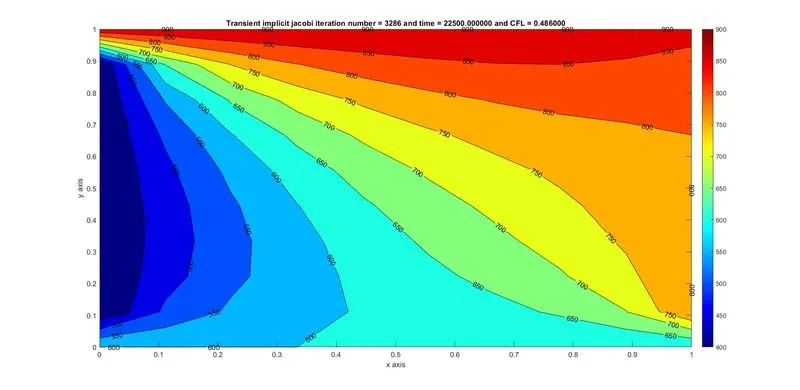
jacobi plot-
figure(6)
gauss seidal plot-
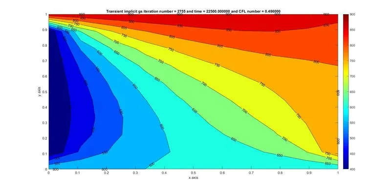
figure(7)
SOR plot-
figure(8)
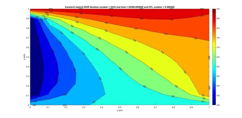
by seeing the plots we can say that the solution reached to steady state condition. to reach the steady state jacobi took 3286 iterations, gauss seidal took 2755 iterations where as SOR took 2523 iterations.
from this we can say SOR technique the solution reached to steady state fast.
SOR plot with CFL number greater than 0.5 :
figure(9)
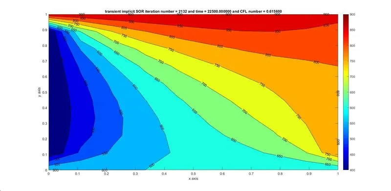
in the above plot the CFL number is 0.615, but the solution didn't gets diverged. and also with less number of iteration the solution reached to steady state compared to CFL number 0.48.
with this we coclude that in transient implicit form, the solution will reamain steady state even after increasing CFL number to greater than 0.5