Week 4.1: Project Steady state simulation of flow over a throttle body

AIM:

Steady state simulation of flow over a throttle body

Objectives:

• Post process the results and show pressure and velocity contours.
• Show the mesh (i.e surface with edges)
• Show the plots for pressure, velocity, mass flow rate and total cell count.
• Create an animation in which it throttle movement should be visible.

theory:

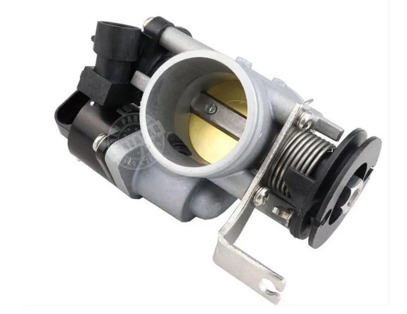
In a traditional spark ignition gasoline engine, the throttle body is the part of the air intake system that controls the amount of air that flows into an engine's combustion chamber. It consists of a housing unit that contains a throttle plate (butterfly valve) that rotates on a shaft. When the accelerator (gas pedal) is pushed down, the throttle plate opens and allows air into the engine. When the gas pedal is released, the butterfly closes and effectively chokes off (throttles) air flow into the combustion chamber. This process effectively controls the speed of the engine and ultimately, the speed of the vehicle.

Geometry:

the below figure is the throttle body with throttle plate.

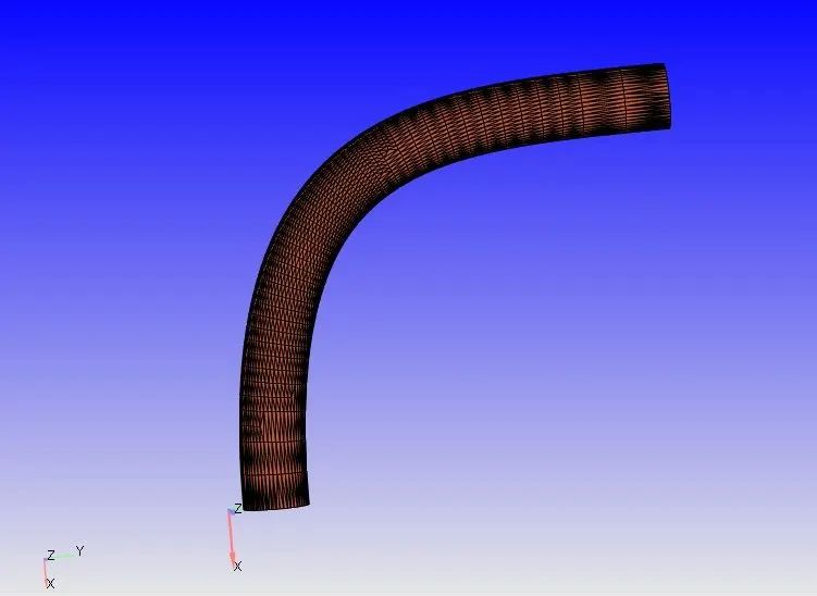
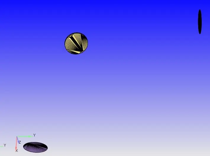
now check the normals of all the faces are facing inside or not by using normal toggle tool and then buid case setup.then i have used boundary tool in the geometry. here i have named the boundaries to the box. i have named the pipe wall as elbow, throotle plate as throttle, inlet and outlet. in the above figure, the top right side face is inlet and the bottem left side face is outlet.

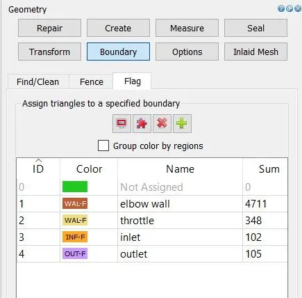
in the above figure, sum represents the number of triangles selected at the each boundary. now use normal toggle tool. in the converge,the normals are aloways directed to outside of the box faces as a default. but here the fluid is inward flow. so eliminate them, click on transform in geometry and slect of triangle and click apply. to check whethere the geometry is correct or not(ie open edges errors, overlap errors), click on the diagnosis which is shown at the bottem left of the display and click findings. mow buid the case setup.

case setup:

application type: time beased

materials: air

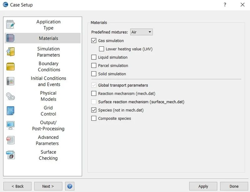
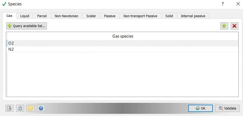
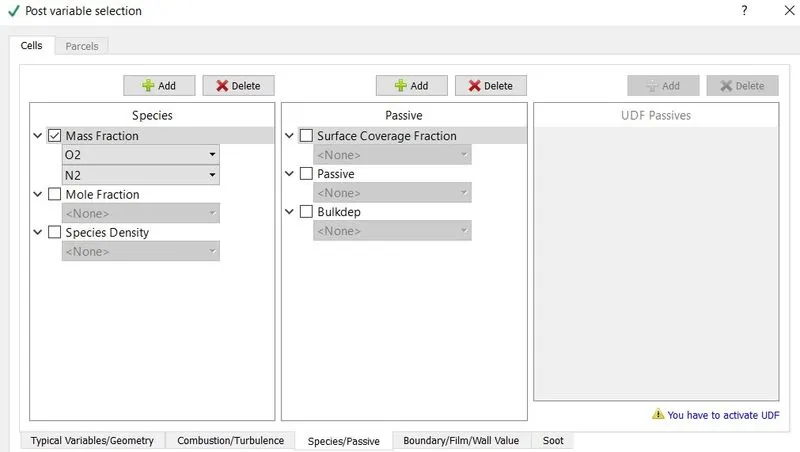
click on gas simulation as the air is gaseous state and click on species to calcuate how the mass fraction of N2 and O2 are changing along the flow.

species-

simulation parameters:

run parameters-

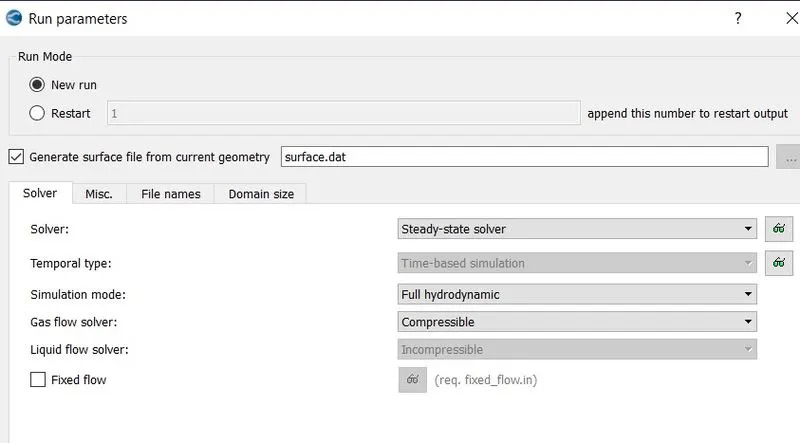
i am running the somulation using steady state solver. here in steady steate condition, the throttle won't move any inclination, so there we be no disturbace for the fluid to flow through the elbow. full hydrodynamic simulation mode is used for simple geometries.

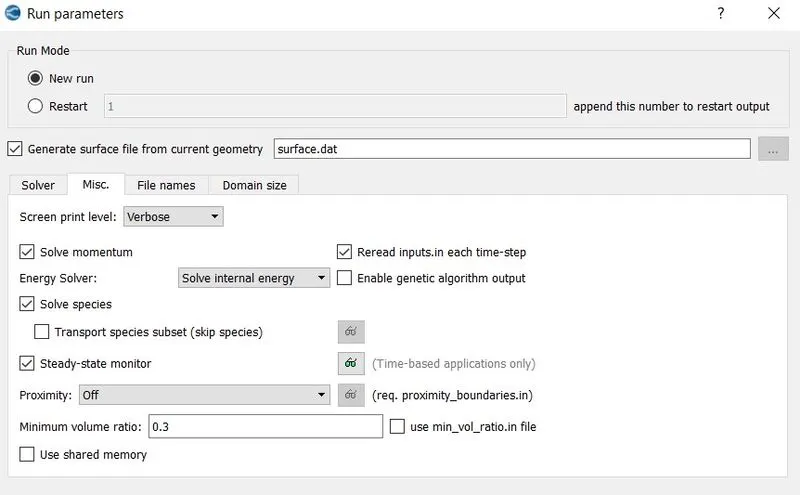
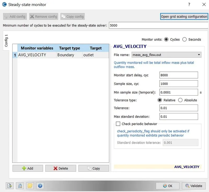
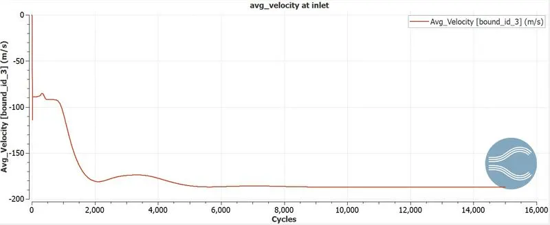
• steady state moniter- it moniters the primitive variables wheather they reached the steady state or not. minimum number of cycles to be executed for steady state solver is 5000. it tells that even if we give the number of cycles to run the simulation at 15000, the software stop calculating the simulation if it reached the steady state in between 5000 and 15000 cycles. moniter start delay indicates the the software start monitoring the simulation whether the solution reached to steady state or not., that is from start. simple size indicates the soft ware takes the solution for every 1000 cycles and compar the difference in changing of primitive varisbles to see whether they reached steady state or not.tolerence denotes the diference in changing of primitive variables at every 1000cycles.

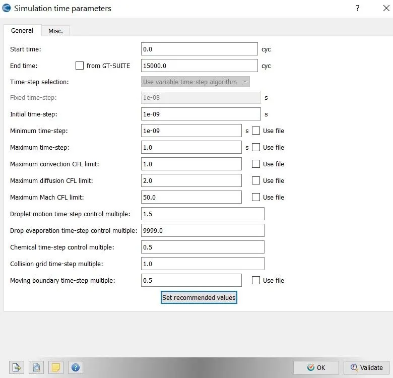
simulation time parameters- the maximum convection cfl number should always be less than or equal to 1. so that solution would converge otherwise solution gets blown up.

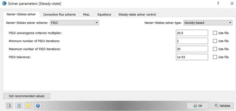
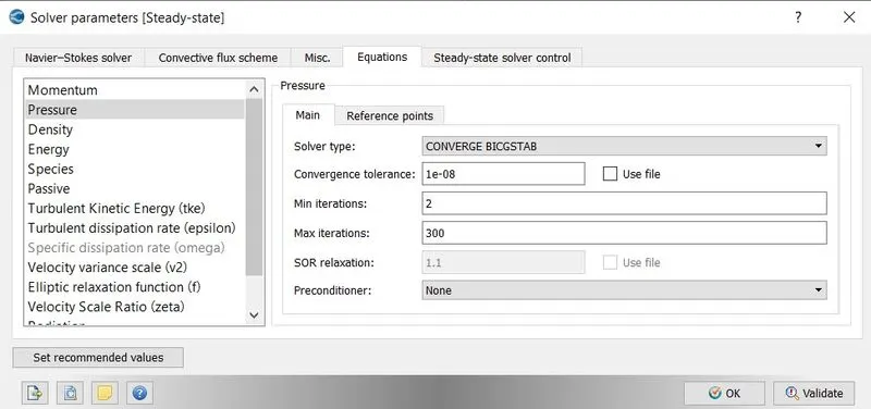
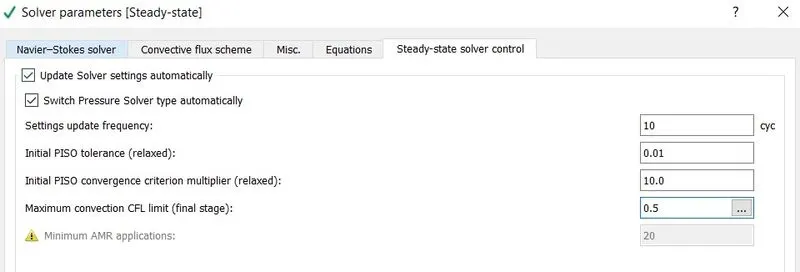
solver parameters-

pressure based solver is used here and the max. cfl number taken is 0.5

initial conditions and events:

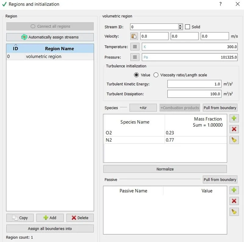
regions and initialization-

here i have named the entire box region as volumetric region.

boundary conditions:

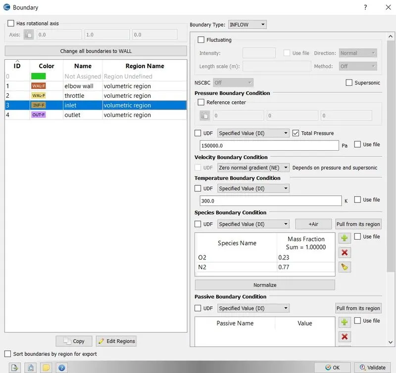
boundary-

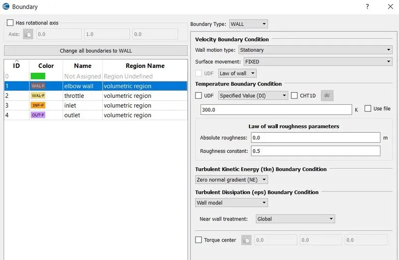
• inlet- the inlet pressure(total pressure) i have taken is 150000 pascals.

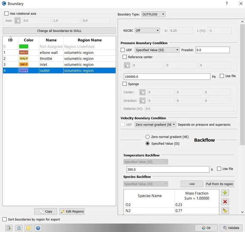
• outlet- the outlet pressure(static pressure) i have taken is 100000 pascals

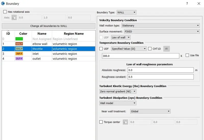
• elbow wall - for the turbulent flows, we have to take law of wall.

• throttle-

physical models:

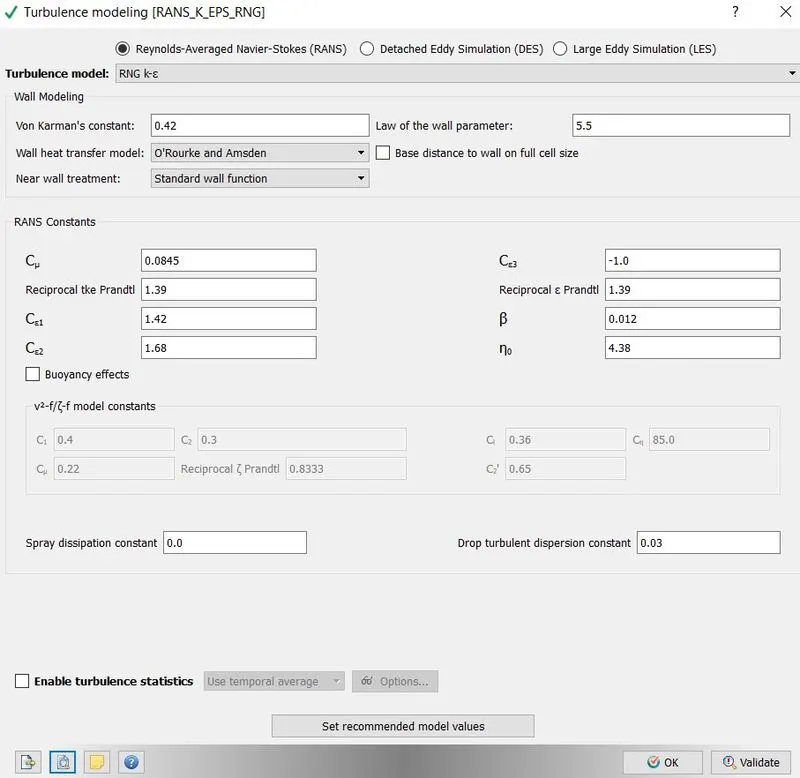
turbulence modelling-

grid control:

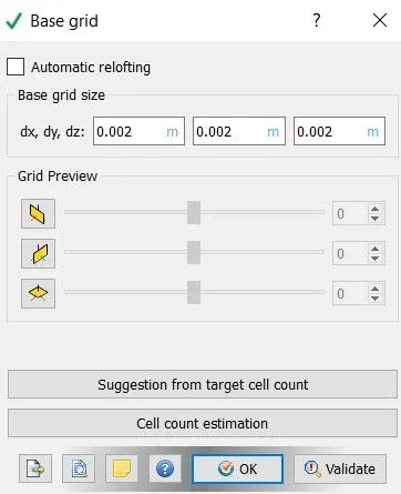
base grid-

fixed embedding-

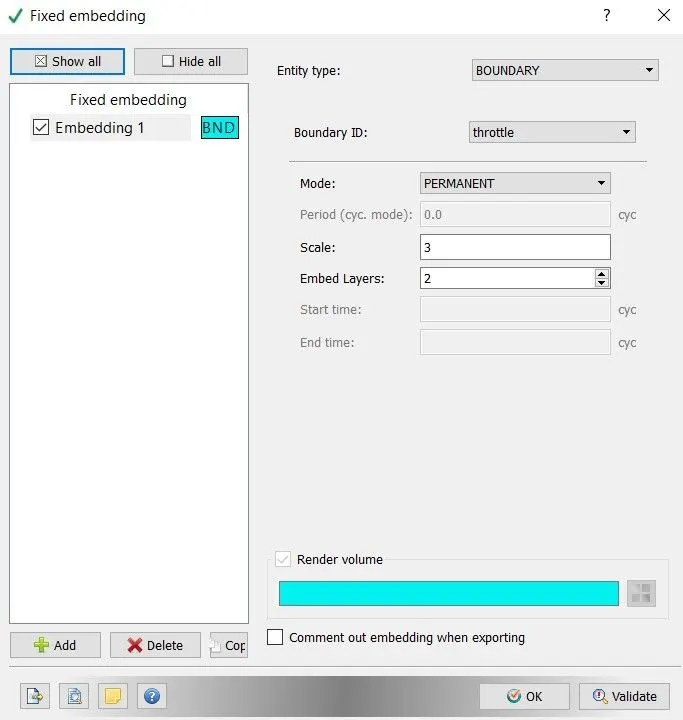
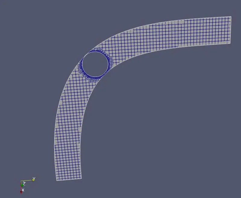
i have enabled fixed embedding because to scale the cells at walls of the geometry. it means to to capture the turbulence in the turbulence boundary layer region, we have to provide cells with small size at the walls of the boundary. embedded layers represents the number of layers of cells we are going to take.

output/post-processing:

post variable selection-

output-

solution:

now export all the input files in a folder. so from this we can see that converge is used to create the input files for the simulation. now insert the two application files from the converge folder to the folder where i have exported all the input files.

for the simulation i have used cygwin64 terminal. in cygwin termpinal open the folder where you have pasted all the input and application files.

now for the simulation write mpiexec.exe -n 4 converge.exe restricted and click enter. here 4 represents the number of processors used at a time.

post processing of results:

for this copy post convert application from converge folder to output folder which is generated in the input files folder. we are doing this because we are goingto convert all the output files into a vtk file which can be easily read by paraview software. toconvert the files we have to use post conver application as shown in the figure. there we can see the results that are obtained. now in cygwin open the output folder and write mpiexec.exe -n 4 post_convert.exe and click enter. now the below figure will appear

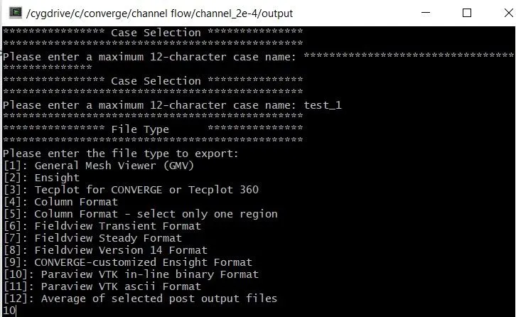
after naming the case and choosing 10, hit enter. now click yes for boundary output surface. now all the output files will appear and then write 'all' to convert all the output files. now select 'all' at cell variable selection menu. now all the files gets converted into paraview vtk files.

now open paraview. in paraview, open file and select case name .. vtm file which is present in the output files. finally we see the geometry in the paraview. now choose slice tool to select the axis along which all the primitive variables are same. as we know that, along z axis the primitive varibles are equal. so select axis and click apply.

mesh:

in the below figure we are seeing the layers around the throttle. this is done because the fluid has to flow in a small gap between the elbow wall and throttle. to visalize the flow in that portion we have increase the cells there. so i have used scale and layer tool in the converge to the throttle.

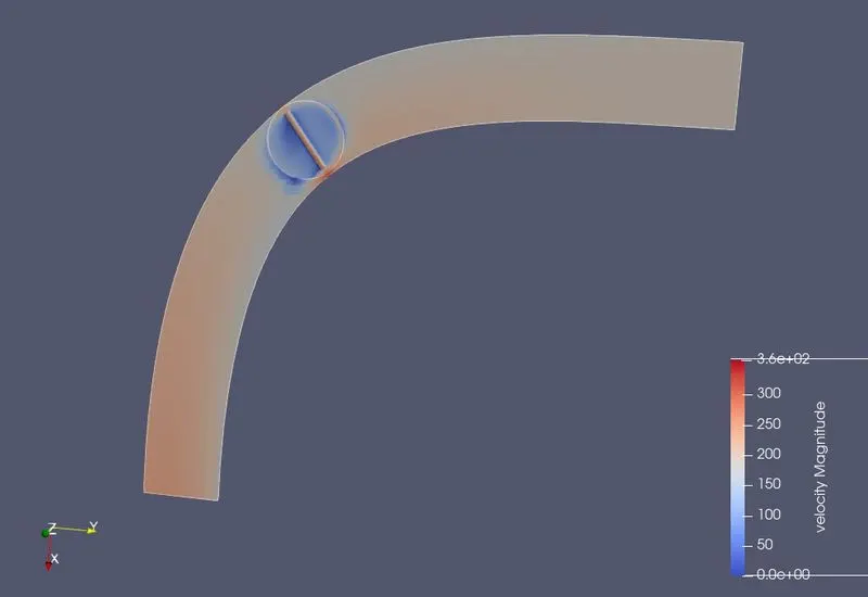
velocity contour-

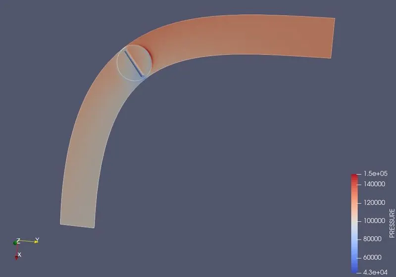
pressure contour-

velocity plot inlet-

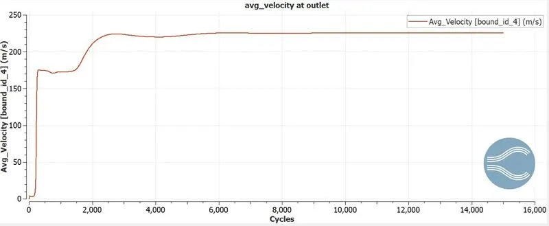
velocity at outlet plot-

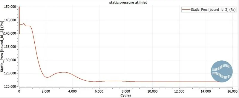
static pressure at inlet plot-

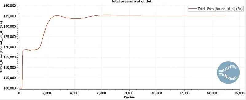
total pressure at outlet-

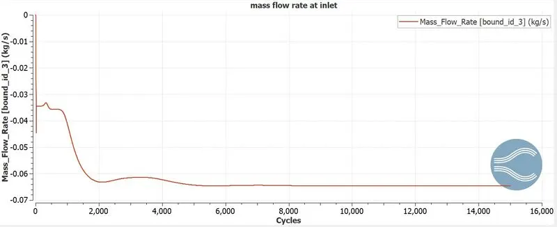
mass flow rate at inlet-

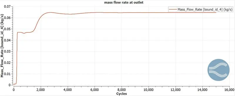
mass flow rate at outlet plot-

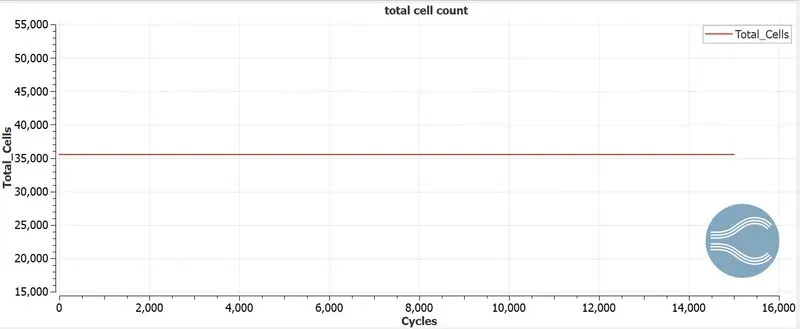
total cell count-

animation for above simulation-

conclusion:

• mass flow rate at inlet and at outlet are constant.
• pressure at ilet is higher compared to outlet, so the fluid can easily move from inlet to outlet.
• steady state simulation is done to observe the magnitude of primitive variables after they gets converged.