Week 3 - Taylor table method and Matlab code
AIM:
Derivation of forth order approximation of second order derivative using taylor table method.
Objective:
here we are going to find the second order derivative,which is evaluated by using numerical approximation methods and then it is going to be compare with exact solution.
Theory:
here we are interested in replacing a partial derivative with a suitable alzebraic difference quotient, i.e., a finite difference. most common finite difference representations of derivatives are based on Taylor table expansion.
higher order approximations:
Order of approxiation tell that how accurate the sollution is obtained while solving the partial differencial equations. in particular, more accurate finite difference quotients can be derived, exhibiting third and forth order accuracy. such higher order accurate difference quotients generally involve information at more grid points than those we have derived.
there are three different schemes are used to obtain second order derivative with forth order accurate quotients.
1. Central difference scheme:
let us assume that the spacing of grid points in the x direction is uniform and given by dx. we are taking the number of grid points using below formula
number of grid points = order of accuracy( also called as order of approximation) + order of derivative + 1.
order of accuracy = 4 and order of derivative = 2
therefore number of grid points we are going to use is 5, with denoting centre grid point as i. from centre we are going to increase the grid points number along right side and decrease the grid point number along left side.
dx dx dx dx
..........|..........|...........|...........|..........|............
i-2 i-1 i i+1 i+2
from the above figure we have divided the domain with 5 grid points with uniform spacing of dx.
let write second order deivative as an equation in central difference scheme,
`(d^2 f)/(dx^2 )= a*f(i-2)+b*f(i-1)+c*f(i)+d*f(i+1)+e*f(i+2)`
to find the values of a,b,c,d,e we are using taylor table method.
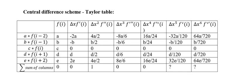
as we are approximating with second order derivative, so we can directly take zero's for f(i), f'(i),f'''(i),f''''(i). we need 5 unknowns so we use only 5 equations.
`a+b+c+d+e = 0`
`-2a-b+d+2e = 0`
`4a+b+d+4e=2/(∆x^2 )` (`dx^2=∆x^2`)
`-8a-b+d+8e=0`
`16a+b+d+16e=0`
by writing the equations in matrix form AX = B, we have values A and B and we are going to obtain the value of X with a,b,c,d,e values.
`a=(-0.0833)/(∆x^2 )` `b=1.333/(∆x^2 )` `c=-2.5/(∆x^2 )` `d=1.333/(∆x^2 )` `e=(-0.0833)/(∆x^2 )`
so the final equation of second order derivative with forth order approximation by using central difference scheme is
`(d^2 f)/(dx^2 )= (-0.0833*f(i-2)+1.333*f(i-1)-2.5*f(i)+1.333*f(i+1)+0.0833*f(i+2))/(∆x^2 )`
2. Skewed right sided difference scheme:
here we are taking number of grid ponits using below formula
number of grid points = order of accuracy( also called as order of approximation) + order of derivative .
order of accuracy = 4 and order of derivative = 2
therefore number of grid points we are going to use is 6, the grid point 'i' denoting at first left place and then grid point number goes on increasing towords right.
dx dx dx dx dx
.......|..........|...........|...........|...........|..........|.......
i i+1 i+2 i+3 i+4 i+5
from the above figure we have divided the domain with 6 grid points with uniform spacing of dx.
let us write second order derivative as an equation in skewed right sided difference scheme,
`(d^2 f)/(dx^2 )= a*f(i)+b*f(i+1)+c*f(i+2)+d*f(i+3)+e*f(i+4)+f*f(i+5)`
to find the values of a,b,c,d,e,f we are going to use taylor table method.
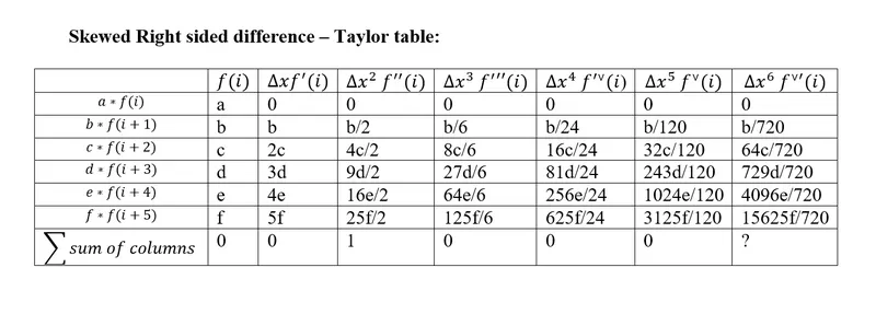
as we are approximating with second order derivative, so we can directly take zero's for f(i), f'(i),f'''(i),f''''(i),f'''''(i). we need 6 unknowns so we use only 6 equations.
`a+b+c+d+e+f=0`
`b+2c+3d+4e+5f=0`
`b+4c+9d+16e+25f=2/(∆x^2 )`
`b+8c+27d+64e+25f =0`
`b+16c+81d+256e+625f=0`
`b+32c+243d+1024e+3125f=0`
by writing the equations in matrix form AX = B, we have values A and B and we are going to obtain the value of X with a,b,c,d,e values.
`a=3.75/(∆x^2 )` `b=-12.833/(∆x^2 )` `c=17.833/(∆x^2 )` `d=-13/(∆x^2 )` `e=5.0833/(∆x^2 )` `f=-0.833/(∆x^2 )`
so the final equation of second order derivative with forth order approximation by using skewed right sided difference scheme is
`(d^2 f)/(dx^2 )= (3.75*f(i)-12.833*f(i+1)+17.833*f(i+2)-13*f(i+3)+5.0833*f(i+4)-0.833*f(i+5))/(∆x^2 )`
3. Skewed left sided difference scheme:
here we are taking number of grid ponits using below formula
number of grid points = order of accuracy( also called as order of approximation) + order of derivative .
order of accuracy = 4 and order of derivative = 2
therefore number of grid points we are going to use is 6, the grid point 'i' denoting at first right place and then grid point number goes on decreases towords left.
dx dx dx dx dx
.......|..........|...........|...........|...........|..........|.......
i-5 i-4 i-3 i-2 i-1 i
from the above figure we have divided the domain with 6 grid points with uniform spacing of dx.
let us write second order derivative as an equation in skewed left sided difference scheme,
`(d^2 f)/(dx^2 )= a*f(i)+b*f(i-1)+c*f(i-2)+d*f(i-3)+e*f(i-4)+f*f(i-5)`
to find the values of a,b,c,d,e,f we are going to use taylor table method.
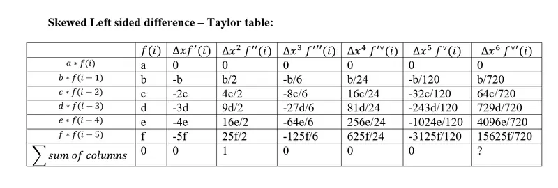
`a+b+c+d+e+f=0`
`b+2c+3d+4e+5f=0`
`b+4c+9d+16e+25f=2/(∆x^2 )`
`b+8c+27d+64e+25f =0`
`b+16c+81d+256e+625f=0`
`b+32c+243d+1024e+3125f=0`
by writing the equations in matrix form AX = B, we have values A and B and we are going to obtain the value of X with a,b,c,d,e values.
`a=3.75/(∆x^2 )` `b=-12.833/(∆x^2 )` `c=17.833/(∆x^2 )` `d=-13/(∆x^2 )` `e=5.0833/(∆x^2 )` `f=-0.833/(∆x^2 )`
so the final equation of second order derivative with forth order approximation by using skewed right sided difference scheme is
`(d^2 f)/(dx^2 )= (3.75*f(i)-12.833*f(i-1)+17.833*f(i-2)-13*f(i-3)+5.0833*f(i-4)-0.833*f(i-5))/(∆x^2 )`
main code:
%discritization of range of dx
clear all
close all
clc

x = pi/3;
%analytical function
analytical_function = exp(x)*cos(x);
dx = linspace(pi/4000,pi/40,20);
for i = 1:length(dx)
    central_difference_error(i) = central_difference(x,dx(i));
    skewed_right_sided_error(i) = skewed_right_difference(x,dx(i));
    skewed_left_sided_error(i) = skewed_left_difference(x,dx(i));
end
loglog(dx,central_difference_error,'r')
hold on
loglog(dx,skewed_right_sided_error,'b')
hold on
loglog(dx,skewed_left_sided_error,'g')
xlabel('dx')
ylabel('error')
legend('central difference','skewed right','skewed left')
function code for central difference scheme-
function  central_difference_error = central_difference(x,dx)

%analytical function
analytical_function = exp(x)*cos(x);
second_order_analytical_derivative = -2*exp(x)*sin(x);
y = [-0.08333333333333333333333333 1.3333333333333333333333333 -2.50 1.333333333333333333333333 -0.083333333333333333333333333];

%central difference scheme of second order derivative = (-0.083f(x-2dx)+1.333f(x-1)-2.5f(x)+1.333f(x+dx)-0.083f(x+2dx))/dx^2
central_difference_second_order = ((y(1)*exp(x-(2*dx))*cos(x-(2*dx)))+(y(2)*exp(x-dx)*cos(x-dx))+(y(3)*exp(x)*cos(x))+(y(4)*exp(x+dx)*cos(x+dx))+(y(5)*exp(x+(2*dx))*cos(x+(2*dx))))/(dx^2);
central_difference_error = abs(central_difference_second_order-second_order_analytical_derivative);
end
function code of skewed right sided difference scheme-
function skewed_right_sided_error = skewed_right_difference(x,dx)

%analytical function
analytical_function = exp(x)*cos(x);
second_order_analytical_derivative = -2*exp(x)*sin(x);
b = [3.75 -12.83333333333333333333333333 17.8333333333333333333333333 -13 5.0833333333333333333333333 -0.833333333333333333333333];
%skewed_right_difference = (3.75*f(x)-12.833f(x+dx)+17.833f(x+2dx)-13f(x+3dx)+5.083f(x+4dx)-0.833f(x+5dx))/dx^2
skewed_right_difference = ((b(1)*exp(x)*cos(x))+(b(2)*exp(x+(1*dx))*cos(x+(1*dx)))+(b(3)*exp(x+(2*dx))*cos(x+(2*dx)))+(b(4)*exp(x+(3*dx))*cos(x+(3*dx)))+(b(5)*exp(x+(4*dx))*cos(x+(4*dx)))+(b(6)*exp(x+(5*dx))*cos(x+(5*dx))))/(dx^2);
skewed_right_sided_error = abs(skewed_right_difference-second_order_analytical_derivative);
end
function code of skewed left sided difference scheme-
function skewed_left_sided_error = skewed_left_difference(x,dx)

%analytical function
analytical_function = exp(x)*cos(x);
second_order_analytical_derivative = -2*exp(x)*sin(x);
z = [3.75 -12.8333333333333333333333 17.8333333333333333333333333 -13 5.0833333333333333333333333 -0.8333333333333333333333333];
%skewed_right_difference = (3.75*f(x)-12.833f(x-dx)+17.833f(x-2dx)-13f(x-3dx)+5.083f(x-4dx)-0.833f(x-5dx))/dx^2
skewed_left_difference = ((z(1)*exp(x)*cos(x))+(z(2)*exp(x-(1*dx))*cos(x-(1*dx)))+(z(3)*exp(x-(2*dx))*cos(x-(2*dx)))+(z(4)*exp(x-(3*dx))*cos(x-(3*dx)))+(z(5)*exp(x-(4*dx))*cos(x-(4*dx)))+(z(6)*exp(x-(5*dx))*cos(x-(5*dx))))/(dx^2);
skewed_left_sided_error = abs(skewed_left_difference-second_order_analytical_derivative);
end
output plot:
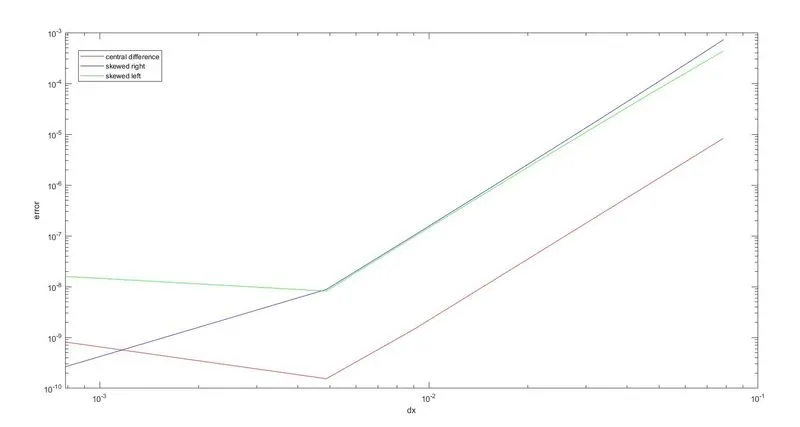
from the plot we have observed that as the dx value increases, central difference scheme showed minimum error compared to skewed right and left difference schemes. so we can use central difference schemes for maximmum values of dx to reduce the error.
error_central difference<error_skewed left difference<error_skewed right difference.
question: why skewed scheme is useful?
ans. skewed schemes are more useful because while solving some complex problems, the numerical stencil not always symmetrical that is the gap between the nodes are not equal, at that time skewed schemes are useful to approximate the numerical complex sollution to analytical solution.
what skewed schems do that central difference cannot do:
in some cases, skewed schmes are more useful compared to central difference schemes, because if we want to calculate error at boundary condtions, central difference schemes cannot find the error beacause at the boundary position there wom't be any node present at either the left or right side of the grid. at that time sckewed schemes give solution accuaretely, as if we want to calculate the boundary position, it can use the all the values either from left side grid points or from right side grid points. if skewed scheme use left side grid points, that scheme is called skewed back sided difference scheme., if the skewed scheme use right side grid points, that sceme is called skewed right sided difference scheme.